Probability and Bayes’ Theorem

Bayesian Statistics - From Concept to Data Analysis

Rahul Saraf

rahul.sarafiitk@gmail.com

zealmaker.com

December 11, 2023

Introduction

Table of Content

1. Introduction

2. Primer to Probability

3. Frameworks of Probability

4. Bayes Theorem

5. Review of Distributions

6. Thank you

7. Background

Preamble

Introduction

What is Statistics?

Statistics is science of uncertainty.

• How do we measure it?
• How do we make decisions in presence of it?
• Quantifiable way to think about uncertainty is to think in terms of probability.

Main Philosophies of Statistics

• Bayesian
• Frequentist

Why do we need Bayesian?

Introduction

Advantages of Bayesian

• Bayesian is better in dealing with uncertainty
  • Ability to quantify uncertainty
  • Combine uncertainties in a coherent manner
• More sensible interpretations of intervals

What is covered in the course?

Introduction

Key Ideas

• Review of few concepts, probability based terms and distributions.

• Review of frequency distributions inference & bayesian inference.

• Priors & Posteriors for discreet distributions : Bernoulli, Binomial & Poisson distributions.

• Continuous distributions - Normal / Gaussian and how to apply it to linear regression.

Coverage

• Difference between bayesian and frequentist inference.

• Key concepts of bayesian inference.

• How to perform bayesian inference on simple cases

Exercises in R and Excel.

Primer to Probability

Table of Content

1. Introduction

2. Primer to Probability

3. Frameworks of Probability

4. Bayes Theorem

5. Review of Distributions

6. Thank you

7. Background

Probability based terms

Primer to Probability

What is an event?

Some outcome that we can potentially or hypothetically observe or experience( e.g. outcome of rolling a fair sided dice)

What is probability?

Chance of an event occurring

What are odds?

• Representation: Event happens: Doesn’t happen (a:b)

• If odd of event B is \[ Odds(B) = \frac{P(B)}{P(B^c)} = a:b \] then -> Probability of event is \(P(B) = \frac{a}{a+b}\)

What are Expectations?

The expected value of a random variable X is a weighted average of values X can take, with weights given by the probabilities of those values .If X can take on only a finite number of values(say, x1, x2,…, xn),we can calculate the expected value as

\[ E(X) = \sum_{i}^{n}(x_i.P(X=x_i)) \]

Rules of Probability

Primer to Probability

• Probabilities must lie between 0 and 1

  \(0 \leq P(A) \leq 1\)

• Probabilities add to 1

  \(\sum_{i=1}^{n}P(X=i) = 1\)

• If A and B are 2 events, the probability that A or B happens(inclusive, either A or B or both)

  \(P(A \cup B) = P(A) + P(B) - P(A \cap B)\)

• For mutually exclusive where only 1 can happen at some point of time.If a set of events \(A_i\) for i = 1,…, m are mutually exclusive then

  \(P(\bigcup^m_{i=1}A_i)=\sum^m_{i=1}P(A_i)\)

Frameworks of Probability

Table of Content

1. Introduction

2. Primer to Probability

3. Frameworks of Probability

4. Bayes Theorem

5. Review of Distributions

6. Thank you

7. Background

Three ways to think

Frameworks of Probability

Classical Framework(CF)

When we have equally likely outcomes or a way to define equally likely outcomes.

Frequentist Framework(FF)

Defines Hypothetical infinite sequence of events. Probability then is relative frequency in that hypothetical infinite sequence of events.

Bayesian Framework(BF)

It takes into account your personal perspective, your measure of uncertainty. It takes into account what you know about a problem ( which may be different from what somebody else believes).

• You can quantify probability by asking the question what is a fair bet.
• If a bet is fair, you should be willing to take it in reverse direction. Expected return from all the outcome is 0.

Some motivating examples

Frameworks of Probability

Example

Notation

1. What is the probability of rolling 4 in a fair dice?

\[ P(x=4)= \frac{1}{6} \]

2. What is the probability of rolling multiple dice such that sum is 4?

\[ P(x_1+x_2=4)=\frac{3}{36} \]

3. What is the probability that the dice is fair?

\[ P(fair) \]

4. What is the probability that it will rain tomorrow?

\[ P(rain_{tomorrow}) \]

5. What is the probability that your internet router will drop a package?

\[ P(drop_{package}) \]

6. What is the probability that router from one provider is more reliable than router from another?

\[ P(Y_1 > Y_2) \]

7. What is the probability that universe will expand forever?

\[ P(universe_{expands}) \]

Examples above requires multiple mindsets to come up with correct interpretation.

Die Problems

Frameworks of Probability

We can consider Section 3.2 examples(1,2,3) either using classical or frequentist paradigm.

Q: What is the probability of rolling 4 in a fair die?

CF

If we each face to be equally likely => Probability if 1/6

FF

Imagine rolling die infinite number of times => Probability then is given by relative frequency of getting 4 which will converge to 1/6 in infinity for fair die.

Q: What is the probability that die is fair?

CF

If only two options are fair and unfair and we consider them equally probable then probability is 0.5.

FF

If die is fair it doesn’t matter how many times we roll it. It will continue to be fair ( or vice versa-> unfair). Hence the probability under this paradigm is either 0 or 1 {0, 1}

Problems in Frequentist Framework

Frameworks of Probability

Q: What is the probability that it will rain tomorrow?

A: Frequentist Framework leads to un-intuitive line of thought here. We need to consider all possible tommorrow and estimate relative frequency of tomorrow where it will rain.

Q: What is the probability that universe will expand forever?

A: Depends on what you believe about the universe.

Deterministic universe

If you believe universe is deterministic, it is either expanding or it is not. This is similar to estimating whether coin is fair or not. Probability is either 0 or 1.

Multiverse

If we believe in multiverse ( many possible universes). Then we have to calculate relative frequency of all universes which are expanding from all the universes in multiverse.

In a nutshell..

Frameworks of Probability

Frequentist Approach

• Frequentist approach tries to be objective in how it defines probabilities.

• Can sometimes run into deep philosophical issues. Sometimes objectivity is just illusory.

• Sometimes we can get interpretations that are not particularily intuitive.

Bayesian Approach

• Subjective approach to probability
• Bayesian Framework + Rules of Probability => Coherence
• If Bet is Fair : Total Expected return should be zero with all the options
• If Total Expected return is not zero/ set up is not coherent then it’s possible for someone to create series of bets which can result in loss for you. This phenomenon is known as Dutch Book

Atacama@Chile : Example

Frameworks of Probability

Q: The country of Chile is divided administratively into 15 regions. The size of the country is 756,096 square kilometers. How big do you think the region of Atacama is?

• Let A1 be the event that Atacama is less than 10,000 square kilometers.

• Let A2 be the event that Atacama is between 10,000 and 50,000 square kilometers.

• Let A3 be the event that Atacama is between 50,000 and 100,000 square kilometers.

• Let A4 be the event that Atacama is more than 100,000 square kilometers.

Atacama@Chile : Solution

Frameworks of Probability

Assign probabilities to A1, A2, A3, A4

In absence of any other evidence, let’s start by assuming all events are equally likely \[ P(A1) = P(A2) = P(A3) = P(A4) = \frac{1}{4} \]

Atacama is the fourth largest of 15 regions. Using this information, revise your probabilities

We don’t know actual probability but intuitively it’s more likely that Atacama is either A3 or A4 bucket. May be we can assign higher probability to them \[ P(A1) = P(A2) = \frac{2}{10}, P(A3) = P(A4) = \frac{3}{10} \]

The smallest region is the capital region, Santiago Metropolitan, which has an area of 15,403 square kilometers. Using this information, revise your probabilities.

Since smallest city is more than limits of A1 bucket. \[ P(A1) = 0 \] Redistributing probability as per remaining proportion \[ P(A2) = \frac{2}{2+3+3}, P(A3) = P(A4) = \frac{3}{2+3+3} \]

The third largest region is Aysén del General Carlos Ibáñez del Campo, which has an area of 108,494 square kilometers. Using this information, revise your probabilities.

This means 4th largest city is definitely less than 108,494. This would probably imply our city is likely to be in A3 bucket. Let’s make A4 zero for now ( to simply calculation) and assign all probability from it to A3

\[ P(A1) = 0 , P(A4) = 0\] Redistributing probability as per remaining proportion \[ P(A2) = \frac{2}{8}, P(A3) = \frac{6}{8} \]

Bayes Theorem

Table of Content

1. Introduction

2. Primer to Probability

3. Frameworks of Probability

4. Bayes Theorem

5. Review of Distributions

6. Thank you

7. Background

Definition

Bayes Theorem

Simple Definition

For two discrete events A & B \[ P(A|B) = \frac{P(A \cap B)}{P(B)} = \frac{P(B|A)P(A)}{P(B|A)P(A)+P(B|{A}^c)P({A}^c)} \]

Three Possible Outcomes (such that exactly one of these must happen)

For 3 discrete events \(A_1\), \(A_2\) and \(A_3\) \[ P({A}_1|B) = \frac{P(B|{A}_1)P({A}_1)}{P(B|{A}_1)P({A}_1)+ P(B|{A}_2)P({A}_2) + P(B|{A}_3)P({A}_3)}\]

General Definition

Events (\(A_1\), \(A_2\) … \(A_m\)) form partition spaces; meaning, Events are mutually exclusive. Exactly one event \(A_i\) must occur and \(\sum_{i=1}^m P(A_i) =1\)

• Discrete Events: \(P({A}_1|B) = \frac{P(B|{A}_1)P({A}_1)}{\sum_{i=1}^mP(B|{A}_i)P({A}_i)}\)
• Continuos Events: \(P({A}_1|B) = \frac{P(B|{A}_1)P({A}_1)}{\int_{i=1}^mP(B|{A}_i)P({A}_i)}\)

Intuition of Bayes theorem and conditional probability

Bayes Theorem

• Bayes theorem is useful when events are related to each other. \(P(A|B)\) or conditional probability of A given B means probability of A happening when B is happening / happened
• We can think about conditional probability as if we are looking at subsegment of problem. We then ask questions about the problem within that subsegment.
• Bayes theorem is used to reverse the direction of conditioning
• A concept of independence is important. If an event A doesnot depend on event B then \(P(A|B)=P(A)\). Under independence condition \(P(A \cap B)=P(A)P(B)\)

Review of Distributions

Table of Content

1. Introduction

2. Primer to Probability

3. Frameworks of Probability

4. Bayes Theorem

5. Review of Distributions

6. Thank you

7. Background

Distributions Definition

Review of Distributions

What is a Random Variable?

Random Variable

A random variable is a quantitative variable whose value depends on chance in some way. Example: We toss the coin 3 times. Then X is a random variable which can take values as {0, 1, 2, 3}. We don’t know what value it will take but it will be one of these 4 values. We can also associate some probabilities to these values

Discrete RV

Can take on Countable number of possible values ( A finite or countably infinite number of possible values)

Some example

• The number of free throws an NBA player makes in his next 20 attempts

  Possible values : 0, 1, 2…, 20

• The number of rolls of a die needed to roll a 3 for first time.

  Possible values: 1, 2, 3 ….

The probability mass distribution of a discrete random variable X is a listing of all possible values of X and their probability of occurring.

Probability Mass Distribution of a coin

Outcome	Probability
H(1)	1/2
T(0)	1/2

Continuous RV

Can take on any value in an interval like number between [4,6] ( An infinite number of possible values)

Mostly variables like height, volume, velocity, weight and time …

Some examples

• The velocity of the ball in cricket [0, \(\infty\)]

• Time between lightning strikes in a thunderstorm

Rules

• For continuous RV probabilities are areas under the curve.So probability at any specific value \(a\) is zero. \(P(x=a)=0\). RV probability is thus practically is defined in an interval of values.\(P(a<x<b)=P(a \leq x \leq b)\)

• \(PDF: f(x)\ge 0 \text{ for all } x\) & \(\int_{-\infty}^{\infty}{f(x)}{dx}=1\)

• \(CDF: F(x) = \int_{-\infty}^x{f(t)}dt\)

Probability distribution: Jaundice example

Review of Distributions : Discrete Distributions

• Approximately 60% of full term newborn babies develop jaundice.

• Suppose we randomly sample 2 full term newborn babies and let \(X\) represent the number that develop jaundice.

What is the probability distribution of \(X\) ?

Possible values: 0, 1, 2

Table 1: Possible outcomes

	JJ	JN	NJ	NN
Value of \(X\)	2	1	1	0
Probability	0.6*0.6	0.6*0.4	0.4*0.6	0.4*0.4

Table 2: Probability distribution of Random variable \(X\) -> \(P(X=x|p)\))

x (Value of \(X\))	0	1	2
p(x)-Probability	0.16	0.48	0.36

Probability distribution: another example representation

Review of Distributions : Discrete Distributions

We can represent (Table 2) as

Probability mass function

\(p(x) = \binom{2}{x} 0.6^x(1-0.6)^{2-x} \text{ for x = 0, 1, 2}\)

\(\text{if x = 0 then } p(x=0) = \binom{2}{0}*0.6^0*0.4^2 = 1*1*0.16= 0.16\)

\(\text{if x = 1 then } p(x=1) = \binom{2}{1}*0.6^1*0.4^1 = 2*0.6*0.4= 0.48\)

\(\text{if x = 2 then } p(x=2) = \binom{2}{2}*0.6^2*0.4^0 = 1*0.36*1= 0.36\)

Histogram

Expectation and Variance of Probability Distribution

Review of Distributions : Discrete Distributions

Expectation/ Expected Value of a random variable

• Theoretical mean of the random variable ( not most likely and many times not been the possible value of random variable \(X\) which can take a value \(x\))

• It is theoretical mean of distribution and not of sample data

• Expectation for \(X\): \(E(X) = \mu = \sum_{\text{all x}}x.p(x)\)

• Expectation of function of \(X\) : \(E(g(X)) = \sum_{\text{all x}}g(x).p(x) \text{ where g(x) is like } x^2, x^3 \text{ or } \sqrt{x}\)

• Law of Large numbers -> As we sample more on more values from the probability distribution. Sample mean will converge to distribution mean.

Variance of X

• \(\sigma^2 = E[(X-\mu)^2] = \sum_{\text{all x}}(x -\mu)^2.p(x)\)
• \(\sigma^2 = E[X^2] -(E(X))^2 = E[X^2] - \mu^2\) ( Relationship holds)

Expectation and Variance of (Table 2) and (@fig-pmf) using above formulae

• \(E(X) = 0*0.16+1*0.48+2*0.36 = 1.2\)
• \(\sigma^2 = 0*0.16+1^2*0.48+2^2*0.36 - 1.2^2= 1.92 -1.44 = 0.48\)

Statistics with Simulation

Review of Distributions : Discrete Distributions

Let \(x\) be value of Random Variable \(X\) and \(sims\) be simulated array of random variables

• Estimating Probabilities

def prob(x, sims):
    m = len(sims)
    return np.sum(sims == x)/ m

• Estimating Cumulative Probability Distribution

def cdf(x, sims):
    m = len(sims)
    return np.sum(sims <= x) / m

• Estimating Probability greater than or equal to certain random value

def pgr(x, sims):
    m = len(sims)
    p = prob(x, sims)
    F = cdf(x, sims)
    return p+1-F # Doing it this way focusses on first entries and eliminates issues with \infinite series

Bernoulli Distribution

Review of Distributions : Discrete Distributions

• Useful when we have 2 possible mutually exclusive outcomes for single trial

  • Success(with probability \(P(Success) = P(X=1) = p\))

  • Failure (with probability \(P(Failure) = P(X=0)=1-p\))

• \(X \sim B(p)\)

• \(PMF : p(X=x|p) = p(x|p) = p^x(1-p)^{1-x}*I_{x \ge 0}(x)\) Here \(I_{x \ge 0}(x)\) is indicator or step function and \(x \in {0,1}\)

• \(E(X) = 1.p^1*(1-p)^0+0.p^0*(1-p)^0 = p+0=p\)

• \(\sigma^2 = E(X^2)-\mu^2 = 1^2p+0^2*(1-p) - p^2= p-p^2 = p(1-p)\)

Examples

• Suppose we toss a fair coin once. What is the distribution of the number of heads?

• Approximately 1 in 200 Indian adults play cricket. If one Indian adult is randomly selected. What is the distribution of cricket playing adult?

Binomial Distribution

Review of Distributions : Discrete Distributions

• \(X \sim Bin(n, p)\) where \(n\) is number of independent bernouli trials and \(p\) is probability of success of any 1 trial. Binomial is number of success in n-independent bernoulli trials
• \(PMF : p(X=x|p, n) = \binom{n}{x}p^x(1-p)^{n-x}\) where \(x \in {0, 1, 2, ... n}\)
• \(E(X) = n\frac{a}{N}\)
• \(Var(X) = \sigma^2 = np(1-p)\)

Examples

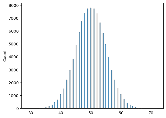
• A coin is flipped 100 times. What is the probability heads comes up at least 60 times?

  \(P(X \ge 60|0.5, 100) \text{ for } x \in {0,1, ..., 100} = BINOM.DIST.RANGE(100, 0.5, 60, 100)= 0.2844\)

• You buy a certain type of lottery ticket once a week for 4 weeks. What is the probability you win a cash prize exactly twice?

  \(P(X=2|p, 4) \text{ for } x \in {0,1,2,3,4} \\ = BINOM.DIST(2,4,p=0.1, FALSE)=0.0486 \\ = COMBIN(4,2)*0.1^2*(1-0.1)^{4-2}=0.0486\)

• A balanced, six-sided die is rolled 3 times. What is the probability a 5 comes up exactly twice?

  \(P(X =2| (p= \frac{1}{6}, 3) \text{ for } x \in {0, 1, 2, 3}=0.069\)

• According to Statistics Canada life tables, the probability a randomly selected 90 year old Canadian male survives for at least another year is approximately 0.82. If 20 => 90 year old Canadian males are randomly selected, what is the probability exactly 18 survive for at-least another year? What is the probability at least 18 survive for at-least another year?

  \(P(X =18|0.82, 20) \text{ for } x \in 0,1,2, …20 = 0.173\)

  \(P(X \ge 18|0.82, 20) \text{ for } x \in 0,1,2, …20 = P(X=18)+P(X=19)+P(X=20)=0.275\)

Simulating Binomial Distribution

Review of Distributions : Discrete Distributions

Simulating Binomial Distribution

def simulate_binomial_rv(p=0.5, n=100, replace=True, m=100000):
    return np.sum(np.random.choice([1, 0], p=[p, 1-p], size=(m, n), replace=replace), axis=1)

sims_binomial = simulate_binomial_rv()
pgr(60, sims_binomial)

0.028730000000000033

Figure 1: Binomial Distribution

Hypergeometric Distribution

Review of Distributions : Discrete Distributions

• Useful when samples are selected( sampling is done) from population without replacement implying that the trials are not independent.

• Probability of success in any individual trial depends on what happened in previous draw.

• \(X \sim Hypgeom(n, a, N)\) where \(n\) objects are chosen without replacement from source that contains \(a\) successes & \(N-a\) failures

• ¹\(PMF : p(X=x|n, a, N) = \frac{\binom{a}{x}\binom{N-a}{n-x}}{\binom{N}{n}}\) where \(x \in Max(0, n-(N-a)), ...Min(a,n)\)

• \(E(X) = n\frac{a}{N}\)

• \(Var(X) = n\frac{a}{N}\frac{N-a}{N}\frac{N-n}{N-1}\)

Example

An urn contains 6 red balls and 14 yellow balls. 5 balls are randomly drawn without replacement. What is the probability exactly 4 red balls are drawn? \(P(X=4)=\frac{\binom{6}{4}\binom{14}{1}}{\binom{20}{5}}=HYPGEOM.DIST(x=4,n=5,a=6,N=20)=0.01354\)

1. If N = 10, a = 7, n = 8 -> \(Max(0, n-(N-a)) = Max(0, 8-3) = 5\) and \(Min(7,8)=7\) implying x can be between 5 to 7. You will at minimum choose 5 successful picks and at max 7 successful picks; every time you pick 8 objects out of 10

Binomial Hypergeometric Equivalence

Review of Distributions : Discrete Distributions

Suppose a large high school has 1100 female students and 900 male students. A random sample of 10 students is drawn. What is the probability exactly 7 of the selected students are female?

• Hypergeometric

\(P(X=4)=\frac{\binom{1100}{7}\binom{900}{3}}{\binom{2000}{10}} \\ =HYPGEOM.DIST(x=7,n=10,a=1100, N=2000) \approx 0.166490\)

• Binomial

\(P(X=4)=\binom{2000}{10}(0.55)^7(1-0.55)^{2000-7} \\ =BINOM.DIST(x=7,n=10,p=\frac{1100}{2000}, FALSE) \approx 0.166478\)

• Sampling rate is \(\frac{n=10}{N=2000}*100=0.5 \%\)

Binomial Distribution can approximate hypergeometric when sampling rate \(\leq\) 5% of population

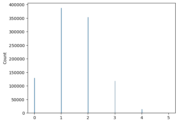
Simulating Hypergeometric Distribution

Review of Distributions : Discrete Distributions

Simulating Binomial Distribution

def simulate_hypergeometric_rv(a, n, N, m=1000000):
    choices = np.hstack([np.ones(a, dtype=int), np.zeros(N-a, dtype=int)])
    # x = np.random.choice(choices, replace=False, size=n) 
    return np.array([np.sum(np.random.choice(choices, replace=False, size=n)) for _ in range(m)])

Figure 2: Hypergeometric Distribution

Geometric Distribution

Review of Distributions : Discrete Distributions

• \(X \sim Geom(x|p)\) -> Distribution of number of trial to get the first success in repeated independent Bernoulli’s trials.

• \(PMF: P(X=x|p) \\ = (1-p)^{x-1}.p \\ \text{where } x \in {1, 2, 3, …,\infty}\)

• ¹\(CDF: F(X=x|p) \\ = \sum_{i=1}^x P(i) = 1-(1-p)^x\)

• \(E(X) = \mu = \frac{1}{p}\)

• \(Var(X) = \sigma^2 = \frac{1-p}{p^2}\)

In a large population of adults, 30% have received CPR training. If adults from this population are randomly selected, what is the probability that the 6th person sampled is the first that has received CPR training?

\(P(X=6) \\= (1-0.3)^5(0.3) \\= 0.050421\)

\(P(X<=6) \\= 1-(1-0.3)^6 \\= 0.882351\)

1. Here intuition is to derive CDF - Use the rule \(\sum_{\text{all x}}P(x) = 1\) , Probability of not succeeding in first x trials = \((1-p)^x\). So cumulative probability to first success up to x trials is subtraction of above terms.

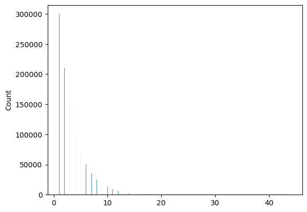
Simulating Geometric Distribution

Review of Distributions : Discrete Distributions

Simulating Geometric Distribution

def simulate_geom_rv(p, m=1000000, cutoff=50):
    s = np.random.choice([1, 0], p=[p, 1-p], size=(m, cutoff)) 
    return np.argmax(s==1, axis=1)+1

Figure 3: Geometric Distribution

Poisson Distribution

Review of Distributions : Discrete Distributions

• Suppose we are counting the number of occurrences of an event in a given unit of time, distance, area or volume like

  • #cars accidents/day
  • #danelions/\(m^2\) plot of land

• Assumptions

  • Events are occurring independently
  • Probability that an event occurs in a given length of time doesn’t change through time.

• Poisson distribution : Distribution of random variable \(X\)[: Number of events in a fixed unit/period of time] given events are occurring randomly and independently, and that the average rate of occurrence is constant.

• \(PMF:P(X=x|\lambda) = \frac{\lambda^xe^{-\lambda}}{x!} \text{ for } x \in 0,1,2,...\infty\)

• \(E(X) = \lambda\)

• \(Var(X) = \lambda\)

• Binomial distribution converges to poisson distribution when \(n \to \infty\) , \(p \to 0\) and \(\lambda = np\) stays constant.

• Or vice versa, poisson distribution approximates binomial distribution if \(n\) is large and \(p\) is small.

Poisson Distribution Example

Review of Distributions : Discrete Distributions

One nanogram of P- 239 will have an average of 2.3 radio-active decays per second, and the number of decays will follow a Poisson distribution

What is the probability that in a 2 second period there are exactly 3 radioactive decays?

\(X\) here is random variable with number of decays in 2 second period.

\(P(X=3|\lambda=4.6)=\frac{4.6^3e^{-4.6}}{3!} \\= POISSON.DIST(3,4.6, FALSE) = 0.1631\)

What is the probability that in a 2 second period there are atmost 3 radioactive decays?

\(P(X\leq3|\lambda=4.6) = POISSON.DIST(3,4.6, TRUE) = 0.3257\)

Negative Binomial Distribution

Review of Distributions : Discrete Distributions

• Distribution of number of bernoulli’s trials to get the \(r^{th}\) success in repeated independent Bernoulli’s trials.

Rules, probabilities and percentile

Review of Distributions : Continuous Distributions

• Suppose for a random variable \(X: f(x) =cx^n \text{ for } a[=2] \leq x \leq b[=4] \text{ and } 0 \text{ otherwise}\). What value of c makes it legitimate probability distribution?

  \(\int_{-\infty}^{\infty} cx^n I_{a \leq x \leq b}{dx} = 1 \implies \int_{a}^{b} cx^n {dx} = 1 \implies c[\frac{x^{n+1}}{n+1}]|_{a}^{b} =1 \implies c = \frac{n+1}{b^{n+1} -a^{n++1}} = \frac{1}{60}\)

• What is \(P(X>k[=3])\) here?

  \(\int_{k}^{\infty} f(x) I_{a \leq x \leq b}{dx} = \int_{k}^{b} cx^n {dx} = c[\frac{x^{n+1}}{n+1}]|_{k}^{b} = \frac{1}{60}[\frac{4^4}{4} - \frac{3^4}{4}] \approx 0.729\)

• What is the median? What is 90-percentile?

  Median: Which splits Area under PDF to 0.5

  \(\\ \implies \int_{-\infty}^{m} f(x) I_{a \leq x \leq b}{dx} = 0.5 \\\implies \int_{a}^{m} f(x){dx} = 0.5 \\\implies \frac{1}{60}[\frac{m^4}{4} - \frac{2^4}{4}] =0.5 \\\implies m = \sqrt[4]{136} \approx 3.41495\)

  Percentile: Which covers 90% Area under PDF

  \(\implies \int_{-\infty}^{m} f(x) I_{a \leq x \leq b}{dx} = 0.9 \\\implies \int_{a}^{m} f(x){dx} = 0.9 \\ \implies \frac{1}{60}[\frac{m^4}{4} - \frac{2^4}{4}] =0.9 \\ \implies m = \sqrt[4]{232} \approx 3.90276\)

• What is the mean and variance?

  Mean: \(\\ E(X) = \int_{-\infty}^{\infty} xf(x) I_{a \leq x \leq b}{dx} \\\implies \int_{a}^{b} xf(x){dx} = \int_{a}^{b} cx^4{dx} \\\implies \frac{1}{60}[\frac{4^5}{5} - \frac{2^5}{5}] \approx 3.3067\)

  Variance: \(\\ E(X^2)-[E(X)]^2 = \int_{-\infty}^{\infty} x^2f(x) I_{a \leq x \leq b}{dx} -\mu^2 \\\implies \int_{a}^{b} x^2f(x){dx} - \mu^2 = \int_{a}^{b} cx^5{dx} - \mu^2 \\\implies \frac{1}{60}[\frac{4^6}{6} - \frac{2^6}{6}] - (3.3067)^2 \approx 0.2657\)

• Some additional Rules

  • \(E(g(x))=\int_{-\infty}^{\infty} g(x)f(x) I_{a \leq x \leq b}{dx}\)
  • Additive: \(E(X+Y) = E(X)+ E(Y)\)
  • Independence: \(\text{if } X\perp Y \text{ then } E(XY) = E(X)E(Y)\)
  • CDF: \(F(x) = P(X\leq x)= \int_{-\infty}^{x} f(t) I_{a \leq t \leq b}{dt} = \int_{a}^{x} f(t){dt} \implies F(x\ge b) = 1\)

Uniform Distribution

Review of Distributions : Continuous Distributions

• \(X \sim U(x|a, b) \text{ for } x \in [a, b]\)

• \(PDF:P(X=x|a,b) = f(x) = cI_{a \leq x \leq b}\)

• To calculate \(c\):\(\int_{-\infty}^{\infty} cI_{a \leq x \leq b}{dx} =1 \implies c = \frac{1}{b-a}\)

• \(E(X)=\mu=\int_{-\infty}^{\infty} cxI_{a \leq x \leq b}{dx} = \int_{a}^{b} cx{dx} = \frac{cx^2}{2}|_a^b = \frac{a+b}{2}\)

• It is a Symmetric Distribution \(\implies median = mean = \frac{a+b}{2}\)

• \(Var(X) = \sigma^2 = E(X^2) - [E(X)]^2 = \int_{a}^{b} cx^2{dx} -\mu^2 = \frac{c(b^3-a^3)}{3} -\mu^2 \\= \frac{a^2+ab+b^2}{3} - \frac{a^2+b^2+2ab}{4} =\frac{a^2+b^2 -2ab}{12} = \frac{(b-a)^2}{12}\)

• \(CDF:F(x) = \int_{-\infty}^{x}c I_{a \leq t \leq b}{dt} = c(x-a) = \frac{x-a}{b-a}\)

• \(P(X>k) = 1-\frac{k-a}{b-a} = \frac{b-k}{b-a}\)

• What is \(n^{th}\)-percentile?

  \(\frac{k-a}{b-a} = \frac{n}{100} \implies k = \frac{n}{100}(b-a) + a\)

Exponential Distribution

Review of Distributions : Continuous Distributions

• \(X \sim Exp(x|\lambda) \text{ for } x \in [0, \infty]\)
• \(PDF:P(X=x|\lambda) = f(x) = \lambda e^{-\lambda x}I_{x >0}\)
• The exponential distribution is a continuous probability distribution that describes the time between events in a Poisson process. A Poisson process is a stochastic process in which events occur randomly in time, but the average rate of occurrence is constant.
• Exponential distribution is the waiting time distribution for a Poisson process.
• \(E(X)=\int_{-\infty}^{\infty}\lambda xe^{-\lambda x}I_{x >0}{dx} = -\frac{1}{\lambda}\int_{-\infty}^{0}ue^{u}{du} = \frac{1}{\lambda}\)
• \(Var(X) = \frac{1}{\lambda^2}\)

Some Applications

• The waiting time between arrivals of customers at a service station can be modeled by an exponential distribution.

• The time between failures of a machine can be modeled by a Poisson distribution.

• The time it takes for a radioactive atom to decay can be modeled by an exponential distribution.

• The number of phone calls received by a call center in a given hour can be modeled by a Poisson distribution.

• The number of hits to a website in a given minute can be modeled by a Poisson distribution.

Thank you

Background

Nutshells

Expandable blocks