Risk Management under Normal Distribution

Imports

library(quantmod)

Loading required package: xts

Loading required package: zoo

Attaching package: 'zoo'

The following objects are masked from 'package:base':

    as.Date, as.Date.numeric

Loading required package: TTR

Registered S3 method overwritten by 'quantmod':
  method            from
  as.zoo.data.frame zoo 

library(ggplot2)
library(purrr) # partial function
library(glue) # string interpolation

RNGkind(sample.kind="Rounding") 

Warning in RNGkind(sample.kind = "Rounding"): non-uniform 'Rounding' sampler
used

set.seed(123789)

GetData

When you click the Render button a document will be generated that includes both content and the output of embedded code. You can embed code like this:

filterSeries <- function(s, date_filter="1979-12-31/2017-12-31", new_name='TR'){
  s <- na.omit(s); s
  s <- s[date_filter]; s
  names(s) <- new_name; s
  return(s)
}

getSeries <- function(name, date_filter="1979-12-31/2017-12-31", src='FRED', new_name='TR'){
  s <- getSymbols(name, src=src, auto.assign = FALSE); s
  s <- filterSeries(s)
  return(s)
}

getSeries("WILL5000IND") |> head(n=3)

             TR
1979-12-31 1.90
1980-01-02 1.86
1980-01-04 1.88

Utility functions

get_df <- function(tbl){
  df <- data.frame(date=index(tbl), TR=as.numeric(tbl$TR))
  return(df)
}

getSeries("WILL5000IND") |> head(n=3) |> get_df()

logret_1 <- function(tbl){
  return(diff(log(tbl))[-1])
}

aggr_fn <-  function(tbl, fn){
  result <- fn(tbl, sum)
  return(result)
}


logret_w <- partial(aggr_fn, fn = apply.weekly)
logret_m <- partial(aggr_fn, fn = apply.monthly)
logret_q <- partial(aggr_fn, fn = apply.quarterly)
logret_a <- partial(aggr_fn, fn = apply.yearly)

ret <- function(logret){
  return(exp(logret)-1)
}

Visualization

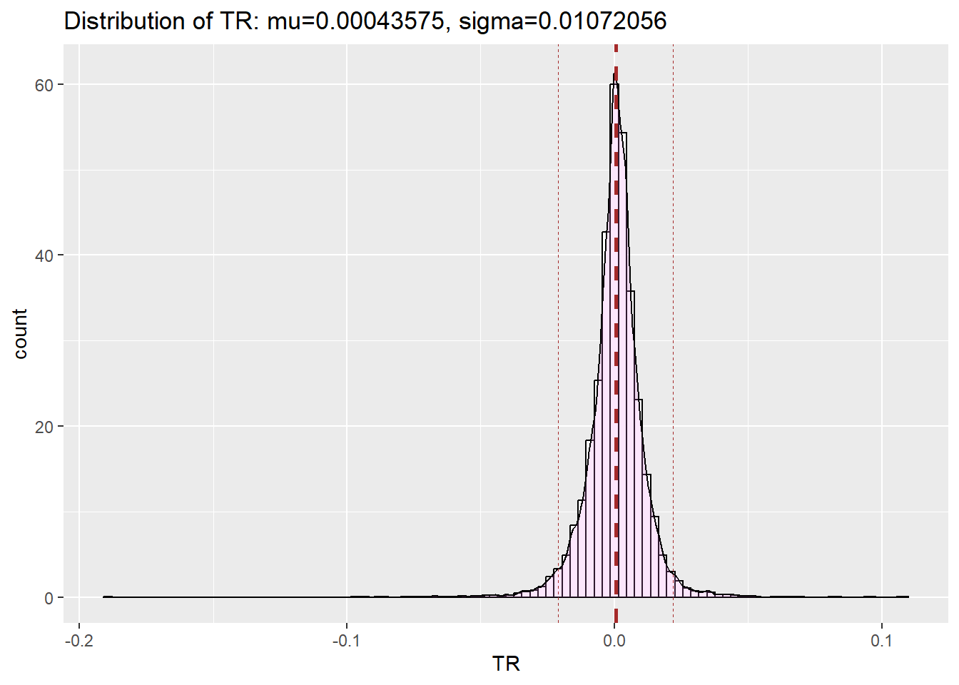
get_dist_plot <- function(tbl){
  mu = mean(tbl)
  sig = sd(tbl)
  p <- get_df(tbl) |> 
    ggplot(mapping = aes(x=TR)) +
    geom_histogram(aes(y=after_stat(density)), colour="black", fill="white", 
                 bins=100)+
    geom_density(alpha=.2, fill="violet") +
    geom_vline(aes(xintercept=mu),
            color="brown", linetype="dashed", linewidth=1) + 
    geom_vline(aes(xintercept=mu+2*sig),
            color="brown", linetype="dashed", linewidth=0.1) +
    geom_vline(aes(xintercept=mu-2*sig),
            color="brown", linetype="dashed", linewidth=0.1) +
    labs(title=glue("Distribution of TR: mu={round(mu, 8)}, sigma={round(sig, 8)}"), y='count')
  return(p)
}

wilsh <- getSeries("WILL5000IND")
wilsh |> 
  logret_1() |> 
  get_dist_plot()

wilsh |> 
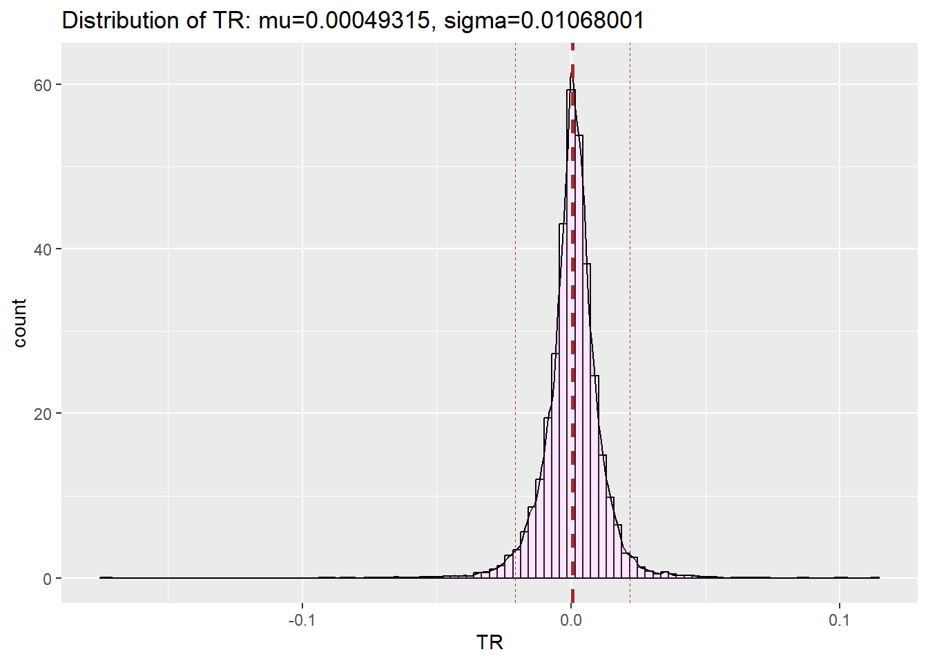
  logret_1() |>
  ret() |> 
  get_dist_plot()

Exercise 5

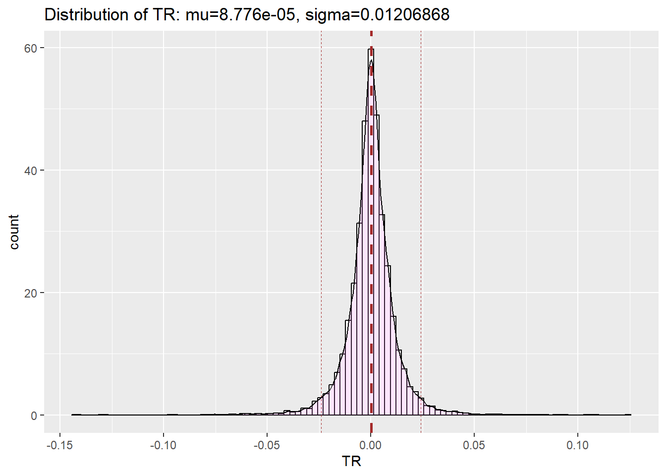
load("W1_Exercise2_FRED_gold.gz"); gold

                TR
1980-01-02  559.50
1980-01-03  634.00
1980-01-04  588.00
1980-01-07  633.50
1980-01-08  610.00
1980-01-09  607.20
1980-01-10  602.85
1980-01-11  623.00
1980-01-14  660.00
1980-01-15  684.00
       ...        
2017-12-12 1240.90
2017-12-13 1242.65
2017-12-14 1251.00
2017-12-15 1254.60
2017-12-18 1260.60
2017-12-19 1260.35
2017-12-20 1264.55
2017-12-21 1264.55
2017-12-27 1279.40
2017-12-28 1291.00

gold |> 
  filterSeries() |> 
  logret_1() |>
  get_dist_plot()

Value-at-Risk(VaR)

• VaR: the amount that a portfolio might lose, with a given probability (1-𝛼), over a given time period.

  • 𝛼 is typically 0.10, 0.05, or 0.01

  • The time period is typically 1 day or 1 week

  • 𝛼 quantile of probability density function

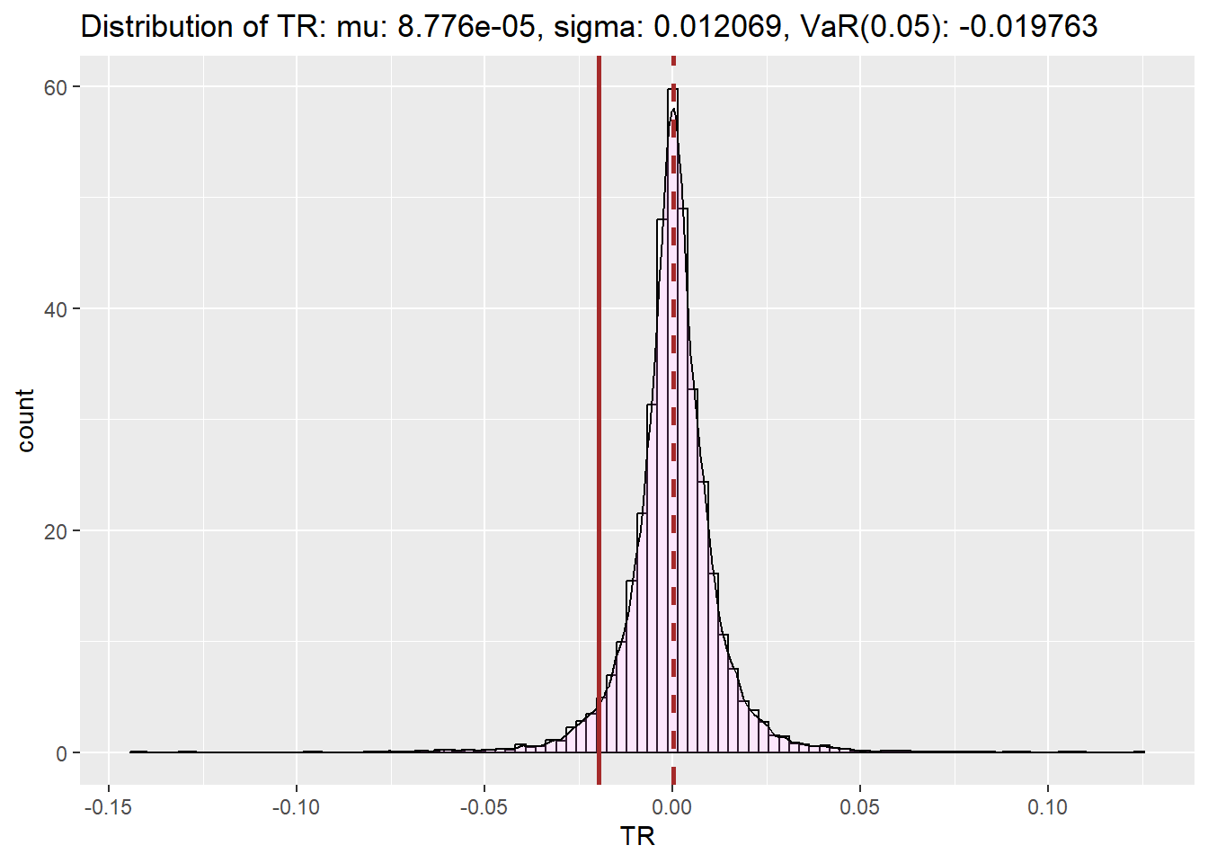
• Example: 𝛼 = 0.05; time period = 1 day. What is the 1-day VaR at the 95% confidence level of the portfolio?

  • Here, the VaR is the maximum loss in the portfolio, over the next trading day, if we exclude the worst 5% of possible outcomes.

get_VaR <- function(tbl,alpha=0.05){
  mu = mean(tbl)
  sig = sd(tbl)
  VaR = qnorm(alpha, mean=mu, sd=sig) #quantile of normal distribution(only not for any other distribution)
  return(VaR)
}

expected_loss <- function(portfolio, risk_num){ #95% confidence that we won't loose more than this amount
  return(portfolio*(exp(risk_num)-1))
}

wilsh |> logret_1() |> get_VaR() |> round(digits=6)

[1] -0.017198

wilsh_VaR <- wilsh |> logret_1() |> get_VaR(); wilsh_VaR

[1] -0.01719801

expected_loss(1000, wilsh_VaR)

[1] -17.05097

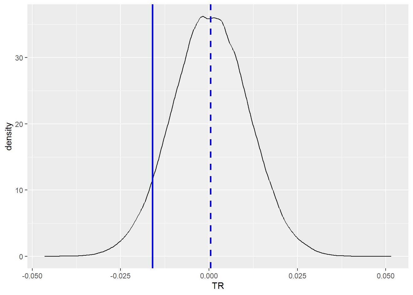
get_VaR_plot <- function(tbl, alpha=0.05){
  mu = mean(tbl)
  sig = sd(tbl)
  VaR = qnorm(alpha, mean=mu, sd=sig)
  p <- get_df(tbl) |> 
    ggplot(mapping = aes(x=TR)) +
    geom_histogram(aes(y=after_stat(density)), colour="black", fill="white", 
                 bins=100)+
    geom_density(alpha=.2, fill="violet") +
    geom_vline(aes(xintercept=mu),
            color="brown", linetype="dashed", linewidth=1) + 
    geom_vline(aes(xintercept=VaR),
            color="brown", linewidth=1) +
    labs(title=glue("Distribution of TR: mu: {round(mu, 8)}, sigma: {round(sig, 6)}, VaR({alpha}): {round(VaR, 6)}"), y='count')
  return(p)
}

wilsh |> 
  logret_1() |> 
  get_VaR_plot()

Exercise 6

load("D:/rahuketu/PPV/S_Self_Study/FinancialRiskManagementR/W1_Exercise2_FRED_gold.gz")
head(gold)

              TR
1980-01-02 559.5
1980-01-03 634.0
1980-01-04 588.0
1980-01-07 633.5
1980-01-08 610.0
1980-01-09 607.2

gold |> 
  filterSeries() |> 
  logret_1() |> 
  get_VaR_plot()

gold_VaR <- gold |> logret_1() |> get_VaR() |> round(digits=6); gold_VaR

[1] -0.019763

expected_loss(1000, gold_VaR) |> round(digits=1)

[1] -19.6

Expected Shortfall (ES)

• Other names

  • conditional value-at-risk (cVaR)

  • average value-at-risk (AVaR)

  • expected tail loss.

• Definition: For the same values of $1 - \alpha$ and time period, expected shortfall (ES) is expected return given that the return is worse than associated VaR.

• In our simple example, a hedge fund has $100 million of investor capital, borrows another $900 million from a bank, and invests the combined $1 billion into the Wilshire 5000 index.

  • What does the 1-day 95% ES tell us?

  • Answer: Over 1 day, if US equities fell by more than the VaR, the hedge fund is expected to lose $21.4 million:

  • $1000 million × [ exp(ES) – 1 ]

get_ES <- function(tbl, alpha=0.05){
  mu = mean(tbl)
  sig = sd(tbl)
  ES = mu - sig*dnorm(qnorm(alpha, mean=0, sd=1), 0, 1)/alpha #quantile of normal distribution(only not for any other distribution)
  return(ES)
}

wilsh_ES <- wilsh |> logret_1() |> get_ES() |> round(digits=6); wilsh_ES

[1] -0.021678

expected_loss(1000, wilsh_ES)

[1] -21.44472

Exercise 7

gold_ES <- gold |> logret_1() |> get_ES() |> round(digits=6); gold_ES

[1] -0.024806

expected_loss(1000, gold_ES) |> round(digits=1)

[1] -24.5

Simulation to Estimate VaR and ES

# get_norm_tbl <- function(mu, sig, n=100000){
#   s <- rnor
# }
n = 10
mu = 0
sig = 1
rnorm(n,mu, sig)

 [1] -0.77986007  0.14633315  1.84487164  0.81671406 -0.76264749 -0.09190092
 [7] -0.86716597  0.96884444  0.64690758  0.42256862

get_norm_series <- function(mu, sig, n=100000){
  RNGkind(sample.kind="Rounding")
  set.seed(123789)
  return(rnorm(n,mu, sig)) 
}
get_norm_series(mu, sig) |> head()

Warning in RNGkind(sample.kind = "Rounding"): non-uniform 'Rounding' sampler
used

[1] -0.77986007  0.14633315  1.84487164  0.81671406 -0.76264749 -0.09190092

get_sim_series <- function(s, n=100000){
  RNGkind(sample.kind="Rounding")
  set.seed(123789)
  return(sample(as.vector(s), n, replace=TRUE))
}

get_sim_series(data.frame(a = 1:3)$a, n=10)

Warning in RNGkind(sample.kind = "Rounding"): non-uniform 'Rounding' sampler
used

 [1] 1 3 2 3 3 2 3 3 1 3

get_sim_VaR <- function(s, alpha=0.05){
  return(quantile(s, alpha) |> unname())
}

s <- get_norm_series(0, 1)

Warning in RNGkind(sample.kind = "Rounding"): non-uniform 'Rounding' sampler
used

VaR <- s |> get_sim_VaR(); VaR

[1] -1.653337

get_sim_ES <- function(s, VaR){
  # VaR  <- get_sim_VaR(s, alpha=alpha)
  return(mean(s[s<VaR]))
}

s |> get_sim_ES(VaR=VaR)

[1] -2.082547

s |> get_VaR()

[1] -1.658957

s |> get_ES()

[1] -2.079746

err <- function(a, b){
  return((a-b)/a*100)
}

a <- s |> get_VaR()
b <- s |> get_sim_VaR()

err(a, b)|> round(digits = 2)

[1] 0.34

s <- wilsh |> logret_1()
VaR <- s |> get_VaR(); VaR

[1] -0.01719801

ES <- s |> get_ES(); ES

[1] -0.02167769

s_sim <- s |> get_sim_series()

Warning in RNGkind(sample.kind = "Rounding"): non-uniform 'Rounding' sampler
used

VaR_sim <-  s_sim|>  get_sim_VaR(); VaR_sim

[1] -0.01602884

ES_sim <- s_sim |> get_sim_ES(VaR=VaR_sim); ES_sim

[1] -0.02528555

err(VaR, VaR_sim) |> round(digits = 2)

[1] 6.8

err(ES, ES_sim) |> round(digits = 2)

[1] -16.64

s <- wilsh |> logret_1()
mu <- mean(s)
sig <- sd(s)
norm_s <- get_norm_series(mu, sig)

Warning in RNGkind(sample.kind = "Rounding"): non-uniform 'Rounding' sampler
used

s_sim <- s |> get_sim_series()

Warning in RNGkind(sample.kind = "Rounding"): non-uniform 'Rounding' sampler
used

VaR <- norm_s |> get_sim_VaR(); VaR

[1] -0.01728895

ES <- norm_s |> get_sim_ES(VaR=VaR); ES

[1] -0.02189033

VaR_sim <-  s_sim|>  get_sim_VaR(); VaR_sim

[1] -0.01602884

ES_sim <- s_sim |> get_sim_ES(VaR=VaR_sim); ES_sim

[1] -0.02528555

err(VaR, VaR_sim) |> round(digits = 2)

[1] 7.29

err(ES, ES_sim) |> round(digits = 2)

[1] -15.51

data.frame(TR=s_sim) |> head()

s <- wilsh |> logret_1()
mu <- mean(s)
sig <- sd(s)
norm_s <- get_norm_series(mu, sig)

Warning in RNGkind(sample.kind = "Rounding"): non-uniform 'Rounding' sampler
used

data.frame(TR=norm_s) |> head()

q <- data.frame(TR=norm_s) |> 
  ggplot(mapping = aes(x=TR)) +
  geom_density(alpha=.2, fill="white") +
  geom_vline(aes(xintercept=mu),
          color="blue", linetype="dashed", linewidth=1) + 
  geom_vline(aes(xintercept=VaR_sim),
          color="blue", linewidth=1)
q

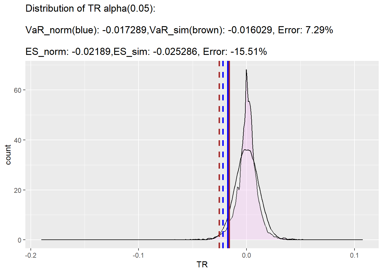
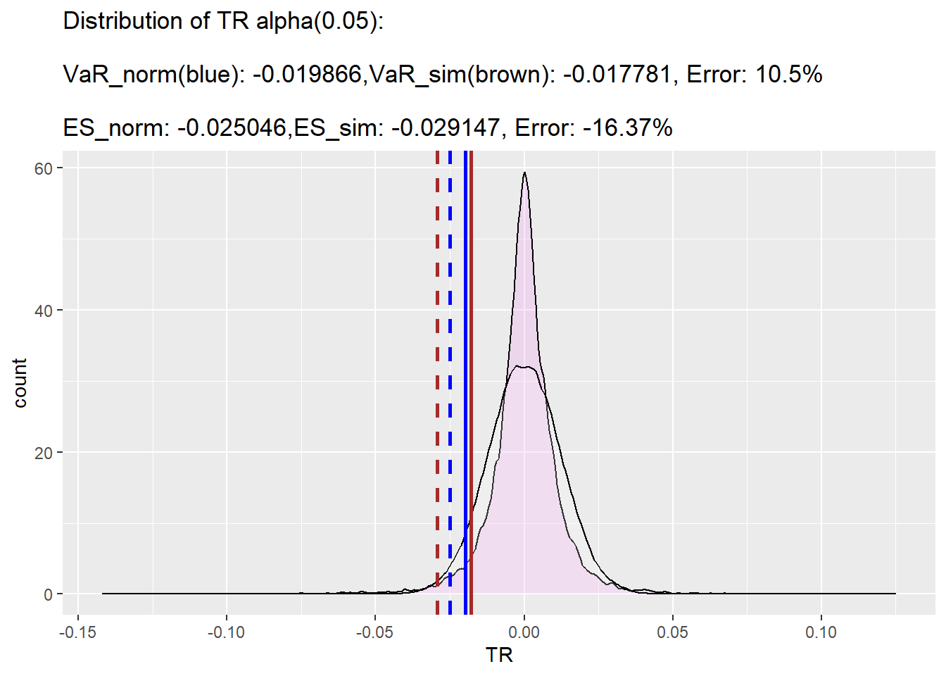
get_comp_plot <- function(s, alpha=0.05){
  mu <- mean(s)
  sig <- sd(s)
  norm_s <- get_norm_series(mu, sig)
  VaR <- norm_s |> get_sim_VaR(); VaR
  ES <- norm_s |> get_sim_ES(VaR=VaR); ES
  s_sim <- s |> get_sim_series()
  VaR_sim <-  s_sim|>  get_sim_VaR(); VaR_sim
  ES_sim <- s_sim |> get_sim_ES(VaR=VaR_sim); ES_sim
  err_VaR <- err(VaR, VaR_sim) |> round(digits = 2)
  err_ES <- err(ES, ES_sim) |> round(digits = 2)

  
  
  p <- data.frame(TR=s_sim, TR2=norm_s) |> 
    ggplot() +
    geom_density(mapping = aes(x=TR), alpha=.2, fill="violet") +
    geom_density(mapping = aes(x=TR2), alpha=.2, fill="white") +
    geom_vline(aes(xintercept=ES_sim),
            color="brown", linetype="dashed", linewidth=1) + 
    geom_vline(aes(xintercept=ES),
            color="blue", linetype="dashed", linewidth=1) + 
    geom_vline(aes(xintercept=VaR_sim),
            color="brown", linewidth=1) +
    geom_vline(aes(xintercept=VaR),
            color="blue", linewidth=1) +
    labs(title=glue("Distribution of TR alpha({alpha}): \n 
                    VaR_norm(blue): {round(VaR, 6)},VaR_sim(brown): {round(VaR_sim, 6)}, Error: {round(err(VaR, VaR_sim), 2)}% \n 
                    ES_norm: {round(ES, 6)},ES_sim: {round(ES_sim, 6)}, Error: {round(err(ES, ES_sim), 2)}%"), y='count')
  return(p)
}

wilsh |> 
  logret_1() |> 
  get_comp_plot()

Warning in RNGkind(sample.kind = "Rounding"): non-uniform 'Rounding' sampler
used

Warning in RNGkind(sample.kind = "Rounding"): non-uniform 'Rounding' sampler
used

Exercise 8

gold |> 
  filterSeries() |> 
  logret_1() |> 
  get_comp_plot()

Warning in RNGkind(sample.kind = "Rounding"): non-uniform 'Rounding' sampler
used

Warning in RNGkind(sample.kind = "Rounding"): non-uniform 'Rounding' sampler
used

set.seed(123789)
s <- gold |> filterSeries() |> logret_1()
mu <- mean(s)
sig <- sd(s)
norm_s <- get_norm_series(mu, sig)

Warning in RNGkind(sample.kind = "Rounding"): non-uniform 'Rounding' sampler
used

s_sim <- s |> get_sim_series()

Warning in RNGkind(sample.kind = "Rounding"): non-uniform 'Rounding' sampler
used

VaR <- norm_s |> get_sim_VaR(); VaR |> round(digits=6)

[1] -0.019866

ES <- norm_s |> get_sim_ES(VaR=VaR); ES |> round(digits=6)

[1] -0.025046

VaR_sim <-  s_sim|>  get_sim_VaR(); VaR_sim |> round(digits=6)

[1] -0.017781

ES_sim <- s_sim |> get_sim_ES(VaR=VaR_sim); ES_sim |> round(digits=6)

[1] -0.029147

err(VaR, VaR_sim) |> round(digits = 2)

[1] 10.5

err(ES, ES_sim) |> round(digits = 2)

[1] -16.37

Quiz 1

us2yen <- getSymbols("DEXJPUS", src='FRED', auto.assign = FALSE)
us2yen <- na.omit(us2yen)
us2yen <- us2yen["1979-12-31/2017-12-31"]
yen2us <- 1/us2yen; yen2us |> head()

               DEXJPUS
1979-12-31 0.004161465
1980-01-02 0.004193751
1980-01-03 0.004195511
1980-01-04 0.004258944
1980-01-07 0.004318722
1980-01-08 0.004259851

set.seed(123789)
s <- yen2us |> logret_1()
mu <- mean(s); mu |> round(digits=6)

[1] 7.9e-05

sig <- sd(s); sig |> round(digits=6)

[1] 0.006756

print("----")

[1] "----"

norm_s <- get_norm_series(mu, sig)

Warning in RNGkind(sample.kind = "Rounding"): non-uniform 'Rounding' sampler
used

s_sim <- s |> get_sim_series()

Warning in RNGkind(sample.kind = "Rounding"): non-uniform 'Rounding' sampler
used

VaR <- s |> get_VaR(alpha=0.01); VaR |> round(digits=6)

[1] -0.015637

ES <- s |>  get_ES(alpha=0.01); ES |> round(digits=6)

[1] -0.017926

print("----")

[1] "----"

VaR_norm <- norm_s |> get_sim_VaR(alpha=0.01); VaR_norm |> round(digits=6)

[1] -0.015816

ES_norm <- norm_s |> get_sim_ES(VaR=VaR_norm); ES_norm |> round(digits=6)

[1] -0.018155

print("----")

[1] "----"

VaR_sim <-  s_sim|>  get_sim_VaR(alpha=0.01); VaR_sim |> round(digits=6)

[1] -0.016872

ES_sim <- s_sim |> get_sim_ES(VaR=VaR_sim); ES_sim |> round(digits=6)

[1] -0.021767

print("----")

[1] "----"

err(VaR_norm, VaR_sim) |> round(digits = 2)

[1] -6.67

err(ES_norm, ES_sim) |> round(digits = 2)

[1] -19.89

expected_loss(1000, ES_sim) |> round(digits=2)

[1] -21.53