Risk Management under Non Normal Distribution

Introduction

Here are a few things covered during this week.

• In real life many distribution are non-normal => We find skewness in distribution of data.
• Distribution of how many cups of coffee some one drinks a day/ alcohol
  • Non drinkers - Data Clustered at zero
  • Low/Moderate drinkers range of usage
  • Addicts/ Alcoholics -Heavy drinkers

• Ways data ( here financial data ) can depart from normality

  • Skewness - right tail $\neq$ left tail [ left skewed if left tail is longer than right tail]

  • Kurtosis - Heaviness of tails of distribution

  • Other ways also exists

• High freq data - daily log returns are typically not normal

• VaR and ES depends on left tail of returns distribution(data) so their value is impacted by nature of distribution.

• What happens when the data / left tails of return is skewed but we assume it’s normal and therefor symmetric.?

  • If distribution is left skewed it has a much longer left tail than symmetric or longer distribution => Large negative returns are more likely in left skewed graph than the middle graph => More negative VaR and ES values.

• What is the implication of heavy tailed distribution on VaR and ES?

  • Large outcomes positive / negative more likely in heavy tailed distribution than normal distribution => VaR and ES will not be correct when assuming normal distribution.

• Test for normality

  • Jarque Bera Test ( JB Static very large with p-value zero -> reject normality

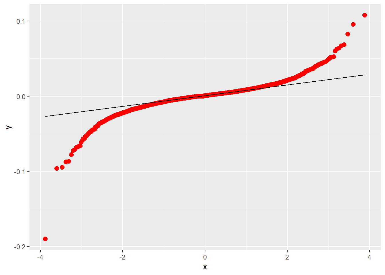
  • QQPlot

  • Kolmogorov-Smirnov Test: Histogram of actual data against histogram of assumed normal distribution

• If data is not normal

  • Find a distribution which describes our data better than the normal distribution

  • In this week we use Student-T Distribution.

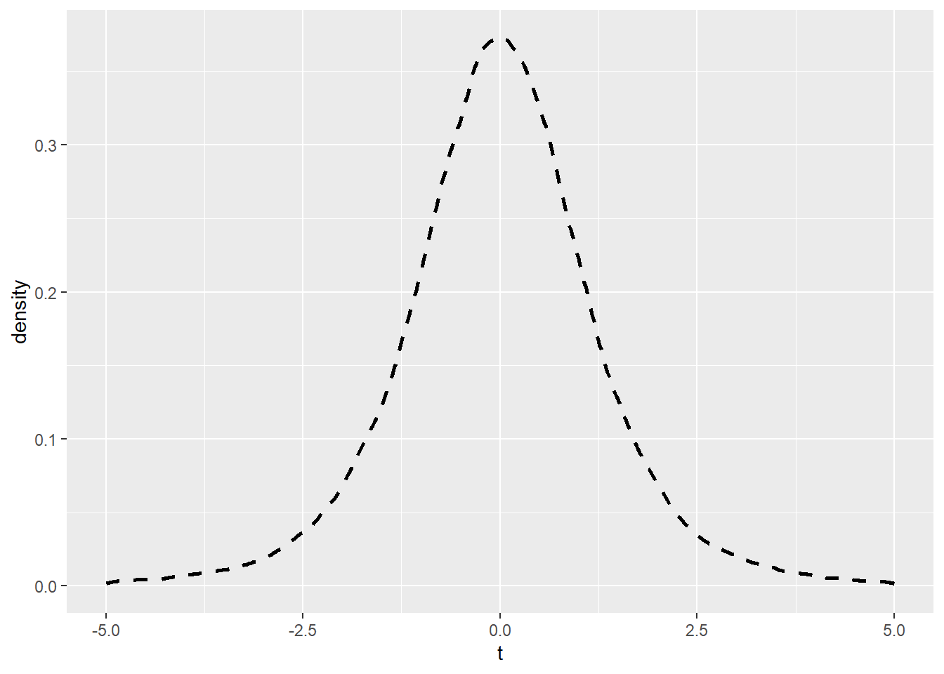
• Student T Distribution

  • Described by mean . sigma and degree of freedom(v)

    • Mean always 0

    • Variance $\frac{v}{v -2} \text{ for } v>2, \infty \text{ for } 1 < v \le 2,\text{ otherwise undefined}$

    • Skewness 0 for v> 3 otherwise undefined

    • Kurtosis 3+ 6/(v-4) for v>4, infinity for 2 < v <= 4, otherwise undefined

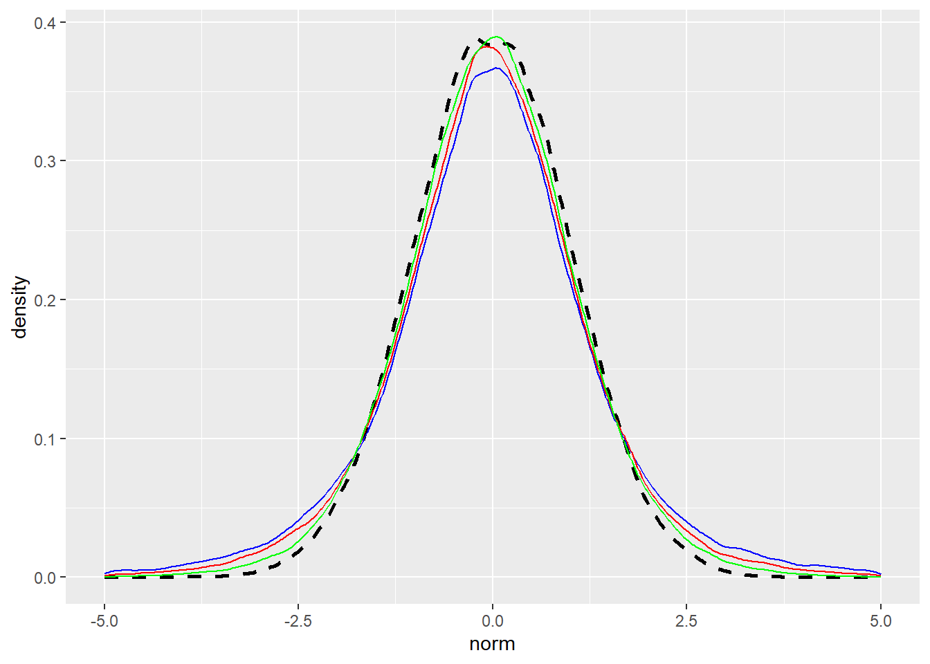
    • At v -> infinity , it is normal distribution.

    • Implies, T-distribution family include normal distribution as a special case.

  • Degree of freedom controls the shape of the distribution

  • Student T- has heavier tail than normal (Kurtosis=3)

  • Differ from normal distribution in term of

    • Same mean and Skewness

    • Differ Std. Dev - not that important

    • Kurtosis is higher

  • Degree of freedom get larger =>Kurtosis get’s smaller.

• How do you match Student-T distribution to data?

  • Problem - Find distribution which match standard deviation and Kurtosis student T distribution to the data.

  • Since we only have single parameter here which is v. We do a trick to solve

    • We need to create 2 equation with 2 unknown => Use Rescaled T-distribution.

    • Divide distribution by root of v/v-2.

    • First find v by matching kurtosis value of data with Rescaled T-Distribution.

    • Pick a scaling parameter to match standard deviation of data.

• Rescaled T-Distribution Model/ Standardized T-Distribution

  • Same mean=0, std. dev=1, skewness=0 as normal distribution. Only difference is kurtosis.

  • Logret = Mean + Standard Deviation * (Rescaled-T distribution with v degrees of freedom).

  • Sigma standard deviation of the data is also known as scaling parameter

  • Statistical test based on MLE to decide which to choose T or normal .[ We can also check by graphing the data]

Imports

library(quantmod)

Loading required package: xts

Loading required package: zoo

Attaching package: 'zoo'

The following objects are masked from 'package:base':

    as.Date, as.Date.numeric

Loading required package: TTR

Registered S3 method overwritten by 'quantmod':
  method            from
  as.zoo.data.frame zoo 

library(ggplot2)
library(purrr) # partial function
library(glue) # string interpolation
library(moments)
library(MASS)
library(metRology)

Attaching package: 'metRology'

The following objects are masked from 'package:base':

    cbind, rbind

Set Seed.

RNGkind(sample.kind="Rounding") 
set.seed(123789)

Functions

filterSeries <- function(s, date_filter="1979-12-31/2017-12-31", new_name='TR'){
  s <- na.omit(s); s
  s <- s[date_filter]; s
  names(s) <- new_name; s
  return(s)
}

getSeries <- function(name, date_filter="1979-12-31/2017-12-31", src='FRED', new_name='TR'){
  s <- getSymbols(name, src=src, auto.assign = FALSE); s
  s <- filterSeries(s)
  return(s)
}

get_df <- function(tbl){
  df <- data.frame(date=index(tbl), TR=as.numeric(tbl$TR))
  return(df)
}

logret_1 <- function(tbl){
  return(diff(log(tbl))[-1])
}

aggr_fn <-  function(tbl, fn){
  result <- fn(tbl, sum)
  return(result)
}

logret_w <- partial(aggr_fn, fn = apply.weekly)
logret_m <- partial(aggr_fn, fn = apply.monthly)
logret_q <- partial(aggr_fn, fn = apply.quarterly)
logret_a <- partial(aggr_fn, fn = apply.yearly)

ret <- function(logret){
  return(exp(logret)-1)
}

get_norm_series <- function(mu, sig, n=100000, set_seed=TRUE){
  if (set_seed){
    RNGkind(sample.kind="Rounding")
    set.seed(123789)
  }

  return(rnorm(n,mu, sig)) 
}

get_sim_series <- function(s, n=100000, set_seed=TRUE){
  if (set_seed){
    RNGkind(sample.kind="Rounding")
    set.seed(123789)
  }

  return(sample(as.vector(s), n, replace=TRUE))
}

get_sim_VaR <- function(s, alpha=0.05){
  return(quantile(s, alpha) |> unname())
}

get_sim_ES <- function(s, VaR){
  # VaR  <- get_sim_VaR(s, alpha=alpha)
  return(mean(s[s<VaR]))
}

get_VaR <- function(tbl,alpha=0.05){
  mu = mean(tbl)
  sig = sd(tbl)
  VaR = qnorm(alpha, mean=mu, sd=sig) #quantile of normal distribution(only not for any other distribution)
  return(VaR)
}

get_ES <- function(tbl, alpha=0.05){
  mu = mean(tbl)
  sig = sd(tbl)
  ES = mu - sig*dnorm(qnorm(alpha, mean=0, sd=1), 0, 1)/alpha #quantile of normal distribution(only not for any other distribution)
  return(ES)
}

expected_loss <- function(portfolio, risk_num){ #95% confidence that we won't loose more than this amount
  return(portfolio*(exp(risk_num)-1))
}

err <- function(a, b){
  return((a-b)/a*100)
}

get_dist_plot <- function(tbl){
  mu = mean(tbl)
  sig = sd(tbl)
  p <- get_df(tbl) |> 
    ggplot(mapping = aes(x=TR)) +
    geom_histogram(aes(y=after_stat(density)), colour="black", fill="white", 
                 bins=100)+
    geom_density(alpha=.2, fill="violet") +
    geom_vline(aes(xintercept=mu),
            color="brown", linetype="dashed", linewidth=1) + 
    geom_vline(aes(xintercept=mu+2*sig),
            color="brown", linetype="dashed", linewidth=0.1) +
    geom_vline(aes(xintercept=mu-2*sig),
            color="brown", linetype="dashed", linewidth=0.1) +
    labs(title=glue("Distribution of TR: mu={round(mu, 8)}, sigma={round(sig, 8)}"), y='count')
  return(p)
}

get_VaR_plot <- function(tbl, alpha=0.05){
  mu = mean(tbl)
  sig = sd(tbl)
  VaR = qnorm(alpha, mean=mu, sd=sig)
  p <- get_df(tbl) |> 
    ggplot(mapping = aes(x=TR)) +
    geom_histogram(aes(y=after_stat(density)), colour="black", fill="white", 
                 bins=100)+
    geom_density(alpha=.2, fill="violet") +
    geom_vline(aes(xintercept=mu),
            color="brown", linetype="dashed", linewidth=1) + 
    geom_vline(aes(xintercept=VaR),
            color="brown", linewidth=1) +
    labs(title=glue("Distribution of TR: mu: {round(mu, 8)}, sigma: {round(sig, 6)}, VaR({alpha}): {round(VaR, 6)}"), y='count')
  return(p)
}

get_comp_plot <- function(s, alpha=0.05){
  mu <- mean(s)
  sig <- sd(s)
  norm_s <- get_norm_series(mu, sig)
  VaR <- norm_s |> get_sim_VaR(); VaR
  ES <- norm_s |> get_sim_ES(VaR=VaR); ES
  s_sim <- s |> get_sim_series()
  VaR_sim <-  s_sim|>  get_sim_VaR(); VaR_sim
  ES_sim <- s_sim |> get_sim_ES(VaR=VaR_sim); ES_sim
  err_VaR <- err(VaR, VaR_sim) |> round(digits = 2)
  err_ES <- err(ES, ES_sim) |> round(digits = 2)

  
  
  p <- data.frame(TR=s_sim, TR2=norm_s) |> 
    ggplot() +
    geom_density(mapping = aes(x=TR), alpha=.2, fill="violet") +
    geom_density(mapping = aes(x=TR2), alpha=.2, fill="white") +
    geom_vline(aes(xintercept=ES_sim),
            color="brown", linetype="dashed", linewidth=1) + 
    geom_vline(aes(xintercept=ES),
            color="blue", linetype="dashed", linewidth=1) + 
    geom_vline(aes(xintercept=VaR_sim),
            color="brown", linewidth=1) +
    geom_vline(aes(xintercept=VaR),
            color="blue", linewidth=1) +
    labs(title=glue("Distribution of TR alpha({alpha}): \n 
                    VaR_norm(blue): {round(VaR, 6)},VaR_sim(brown): {round(VaR_sim, 6)}, Error: {round(err(VaR, VaR_sim), 2)}% \n 
                    ES_norm: {round(ES, 6)},ES_sim: {round(ES_sim, 6)}, Error: {round(err(ES, ES_sim), 2)}%"), y='count')
  return(p)
}

Skewness

• sk = 0 - symmetric

• sk < 0 - left skewed

• sk > 0 - right skewed

wilsh <- getSeries("WILL5000IND"); wilsh

               TR
1979-12-31   1.90
1980-01-02   1.86
1980-01-04   1.88
1980-01-07   1.89
1980-01-08   1.93
1980-01-09   1.93
1980-01-10   1.95
1980-01-11   1.95
1980-01-14   1.96
1980-01-15   1.97
       ...       
2017-12-15 123.53
2017-12-18 124.31
2017-12-19 123.85
2017-12-20 123.80
2017-12-21 124.10
2017-12-22 124.03
2017-12-26 123.94
2017-12-27 124.04
2017-12-28 124.33
2017-12-29 123.67

wilsh |> logret_1() |> as.vector() |> skewness() |> round(digits=2)

[1] -0.91

wilsh |>  head()

             TR
1979-12-31 1.90
1980-01-02 1.86
1980-01-04 1.88
1980-01-07 1.89
1980-01-08 1.93
1980-01-09 1.93

Kurtosis

• normal(3)

• thin-tailed(<3)

• heavy-tailed(>3)

• Usually we have heavy-tailed not thin-tailed

wilsh |> logret_1() |> as.vector() |> kurtosis() |> round(digits=2)

[1] 21.8

Jarque-Berra test for normality

wilsh |> logret_1() |> as.vector() |> jarque.test()

    Jarque-Bera Normality Test

data:  as.vector(logret_1(wilsh))
JB = 142514, p-value < 2.2e-16
alternative hypothesis: greater

Reject normality if p-value is very small.

Kilmogorov Smrinoff test for normality

Todo:: Visual is get_comp_plot

QQPlot

wilsh |> 
  logret_1() |> 
  get_df() |> 
  ggplot(mapping = aes(sample=TR)) +
  stat_qq(size=2.5, color='red') +
  stat_qq_line()

• Synopsis for Wilshire 5000

  • Daily log return of Wilshire 5000 (Left skewed, heavy tailed and non normal)

  • Implication we should estimated VaR and ES without assuming normality.

Exercise 9

load("W1_Exercise2_FRED_gold.gz")

g <- gold |> filterSeries() |> logret_1()

g |> as.vector() |> skewness() |> round(digits=2)

[1] -0.09

g |> as.vector() |> kurtosis() |> round(digits=2)

[1] 15.43

g |> as.vector() |> jarque.test()

    Jarque-Bera Normality Test

data:  as.vector(g)
JB = 61330, p-value < 2.2e-16
alternative hypothesis: greater

g <- wilsh |> logret_1()

g |> as.vector() |> skewness() |> round(digits=2)

[1] -0.91

g |> as.vector() |> kurtosis() |> round(digits=2)

[1] 21.8

g |> as.vector() |> jarque.test()

    Jarque-Bera Normality Test

data:  as.vector(g)
JB = 142514, p-value < 2.2e-16
alternative hypothesis: greater

Student-T Distribution(Rescaled)

t_v3 <- rt.scaled(100000,mean=0,sd=1,df=3) 
t_v5 <- rt.scaled(100000,mean=0,sd=1,df=5)
t_v10 <- rt.scaled(100000,mean=0,sd=1,df=10)
norm <- get_norm_series(0,1)
data.frame(v3=t_v3, v5=t_v5, v10=t_v10, norm=norm) |> 
 ggplot() + 
 geom_density(mapping = aes(x=norm), linetype="dashed", linewidth=1) + 
 geom_density(mapping = aes(x=v3), color='blue') +
 geom_density(mapping = aes(x=v5), color='red') +
 geom_density(mapping = aes(x=v10), color='green') +
 xlim(-5,5) +
 theme(legend.position="top")

#| warning: false
get_t_series <- function(mu, sig, df, n=100000, set_seed=TRUE){
  if (set_seed){
    RNGkind(sample.kind="Rounding")
    set.seed(123789)
  }
  return(rt.scaled(n,mean=mu,sd=sig,df=df)) 
}


t_series <- get_t_series(0,1,4)

Warning in RNGkind(sample.kind = "Rounding"): non-uniform 'Rounding' sampler
used

data.frame(t=t_series) |> 
 ggplot() + 
 geom_density(mapping = aes(x=t), linetype="dashed", linewidth=1) + 
 xlim(-5,5) +
 theme(legend.position="top")

Warning: Removed 741 rows containing non-finite values (`stat_density()`).

get_norm_series_from_s <- function(s, n=100000, set_seed=TRUE){
  mu = mean(s)
  sig = sd(s)
  return(get_norm_series(mu, sig, n=n, set_seed = set_seed))
}

wilsh |> logret_1() |> get_norm_series_from_s() |> head()

[1] -0.0079247909  0.0020045205  0.0202138069  0.0091913802 -0.0077402624
[6] -0.0005494825

get_fit_params  <- function(s){
  fitpars <- s |> as.vector() |> fitdistr(densfun='t') 
  return(fitpars)
}

get_t_series_from_s <- function(s, n=100000, fitpars=NULL, set_seed=TRUE){
  if(is.null(fitpars)){
    fitpars <- s |> get_fit_params()
  }
  t.fit <- fitpars
  return(get_t_series(mu=t.fit$estimate[1], 
                      sig=t.fit$estimate[2], 
                      df=t.fit$estimate[3], 
                      n=n, 
                      set_seed=set_seed))
}

wilsh |> logret_1() |> get_t_series_from_s() |> head()

[1] -0.005139343  0.011403841 -0.005720739  0.002640338  0.004162427
[6] -0.007797006

do_analysis <-  function(s, alpha=0.05){
 
  modelname1 <-  "Norm"
  VaR1 <- s |> get_VaR() |> as.double()
  ES1 <- s |> get_ES() |> as.double()
  # df[nrow(df) + 1,] <- c(modelname, VaR, ES)
  
  modelname2 <-  "NormSim"
  norm_series <- s |> get_norm_series_from_s() 
  VaR2 <- norm_series|> get_sim_VaR(alpha=alpha) |> as.double()
  ES2 <- norm_series |> get_sim_ES(VaR=VaR2) |> as.double()
  # df[nrow(df) + 1,] <- c(modelname, VaR, ES)
  
  modelname3 <-  "T-Sim"
  t_series <- s |> get_t_series_from_s()
  VaR3 <- t_series|> get_sim_VaR(alpha=alpha) |> as.double()
  ES3 <- t_series |> get_sim_ES(VaR=VaR3) |> as.double()
  # df[nrow(df) + 1,] <- c(modelname, VaR, ES)
  
  modelname4 <-  "Sim"
  sim_series <- s |> get_sim_series() 
  VaR4 <- sim_series|> get_sim_VaR(alpha=alpha) |> as.double()
  ES4 <- sim_series |> get_sim_ES(VaR=VaR4) |> as.double()
  
  model_names <- c(modelname1, modelname2, modelname3, modelname4)
  VaRs <- c(VaR1, VaR2, VaR3, VaR4)
  ESs <- c(ES1, ES2, ES3, ES4)

  return(data.frame(ModelName=model_names, VaR=VaRs, ES=ESs))
  
}



wilsh |> logret_1() |> do_analysis(alpha=0.05) |> format(digits = 5)

expected_loss_df <- function(df, portfolio=1000){
  expected_loss_port = partial(expected_loss, portfolio=portfolio)
  df$VaR <- sapply(df$VaR, expected_loss_port)
  df$ES <- sapply(df$ES, expected_loss_port)
  return(df)
}

df <- wilsh |> logret_1() |> do_analysis(alpha=0.05) |> expected_loss_df()
df |> format(digits=4)

Exercise 10

g <- gold |> filterSeries() |> logret_1()
t.fit <- g |> as.vector() |> fitdistr(densfun='t'); t.fit

        m              s              df     
  1.665751e-04   8.001998e-03   4.799590e+00 
 (9.373677e-05) (         NaN) (         NaN)

t.fit$estimate[1] |> round(digits=6)

       m 
0.000167 

t.fit$estimate[2] |> round(digits=6)

       s 
0.008002 

t.fit$estimate[3] |> round(digits=8)

     df 
4.79959 

g |> do_analysis(alpha=0.05) |> format(digits = 5)

VaR and ES for multi-day horizon

• Simple principle: Calculate n (10)- 1 day returns from logret_1 and add them together to get n(10) days return.

• We need to understand / check for time dependence - Block vs iid draws

• Methods

  • Simulate from estimated student - t distribution

  • Simulate from empirical distribution with iid draws

  • Simulate from empirical distribution with block draws(This takes into account time dependence between daily return if any)

Multi day Horizon ( T-Dist/IID)

get_multi_day_series <- function(s, 
                                 days=10, 
                                 sampling_func=get_sim_series, 
                                 n=100000, 
                                 set_seed=TRUE){
  
  if (set_seed){
    RNGkind(sample.kind="Rounding")
    set.seed(123789)
  }

  rvec <- rep(0, n)
  for( i in 1:days){
    rvec <- rvec + sampling_func(s=s, n=n, set_seed=FALSE)
    # print(rvec |> head())
  }
  return(rvec)
}

wilsh |> logret_1() |> get_multi_day_series() |> head()

[1]  0.031583146  0.059921921  0.021241954  0.070948242  0.005151238
[6] -0.004814838

rvec <- wilsh |> logret_1()
s <-  rvec |> get_multi_day_series()
VaR <- s |> get_sim_VaR(alpha=0.05); VaR

[1] -0.05115037

ES <- s |> get_sim_ES(VaR=VaR);ES

[1] -0.07293501

rvec <- wilsh |> logret_1()
fitspars <- rvec |> get_fit_params() #; fitspars
sampling_func_tdist <-  partial(get_t_series_from_s, fitpars = fitspars);  
s <-  rvec |> get_multi_day_series(sampling_func = sampling_func_tdist)
VaR <- s |> get_sim_VaR(alpha=0.05); VaR

[1] -0.04779436

ES <- s |> get_sim_ES(VaR=VaR);ES

[1] -0.07050687

Block Simulation

Steps

• Get a block size of n-days

• Calculate logret_ndays

• get_sim_series for logret_ndays

tbl <- wilsh |> logret_1()
tbl[1:10]

                     TR
1980-01-02 -0.021277398
1980-01-04  0.010695289
1980-01-07  0.005305052
1980-01-08  0.020943174
1980-01-09  0.000000000
1980-01-10  0.010309370
1980-01-11  0.000000000
1980-01-14  0.005115101
1980-01-15  0.005089070
1980-01-16  0.000000000

posn <- 3
days <- 10

sum(tbl[posn:(posn+days-1)])

[1] 0.04676177

tbl <- wilsh |> logret_1()
days <- 10
sapply(seq(1:(nrow(tbl)-days+1)), function(i){
 sum(tbl[i:(i+days-1)])
}) |> head()

[1] 0.03617966 0.05745706 0.04676177 0.05155781 0.02557684 0.04061472

logret_ndays <- function(tbl, days=10){
  len_tbl <-  (nrow(tbl)-days+1)
  new_TR <- sapply(seq(1:len_tbl), function(i){
    sum(tbl[i:(i+days-1)])
    })
  tbl[1:len_tbl]$TR <- new_TR
  return(tbl[1:len_tbl])
}

logret_ndays(tbl) |> length()

[1] 9574

tbl |> length()

[1] 9583

s <- wilsh |> logret_1() |> logret_ndays(days=10) |> get_sim_series()
VaR <- s |> get_sim_VaR(alpha=0.05); VaR

[1] -0.04700005

ES <- s |> get_sim_ES(VaR=VaR); ES

[1] -0.07780043

This is probably a nicer way to simulate block based simulation first by calculating logret_10 and then simulating the regular series. Only challenge is because of randomness, we can’t match results with exactly with random number seed process. So let’s implement a block based approach that exactly matches our answer from presentation.

get_multi_day_series_block <- function(s,
                                       days=10, 
                                       n=100000, 
                                       set_seed=TRUE){
  
  if (set_seed){
    RNGkind(sample.kind="Rounding")
    set.seed(123789)
  }
  rdat <- s |> as.vector()
  rvec <- rep(0, n)
  posn <- seq(from=1, to=(length(rdat)-days+1), by=1)
  rpos <- sample(posn, size=n, replace=TRUE)
  for( i in 1:days){
    rvec <- rvec + rdat[rpos]
    rpos <- rpos+1 
  }
  return(rvec)
}




rvec <- wilsh |> logret_1()
s <-  rvec |> get_multi_day_series_block(days=10)
VaR <- s |> get_sim_VaR(alpha=0.05); VaR

[1] -0.04700005

ES <- s |> get_sim_ES(VaR=VaR);ES

[1] -0.07780043

This matches our last answer. Perhaps answer in ppt is not correct?

do_multi_analysis <-  function(rvec, days=10,  alpha=0.05){
  
  modelname1 <-  glue("student-t({days})")
  fitspars <- rvec |> get_fit_params() #; fitspars
  sampling_func_tdist <-  partial(get_t_series_from_s, 
                                  fitpars = fitspars)
  s1 <-  rvec |> get_multi_day_series(
    sampling_func=sampling_func_tdist)
  VaR1 <- s1 |> get_sim_VaR(alpha=alpha) |> as.double()
  ES1 <- s1 |> get_sim_ES(VaR=VaR1) |> as.double()
  
  modelname2 <-  glue("IID({days})")
  s2 <-  rvec |> get_multi_day_series(days=days)
  VaR2 <- s2 |> get_sim_VaR(alpha=alpha) |> as.double()
  ES2 <- s2 |> get_sim_ES(VaR=VaR2) |> as.double()
  
  modelname3 <-  glue("consecutive({days})")
  s3 <-  rvec |> logret_ndays(days=days) |> get_sim_series(set_seed = TRUE)
  VaR3 <- s3 |> get_sim_VaR(alpha=alpha) |> as.double()
  ES3 <- s3 |> get_sim_ES(VaR=VaR3) |> as.double()
  
  model_names <- c(modelname1, modelname2, modelname3)
  VaRs <- c(VaR1, VaR2, VaR3)
  ESs <- c(ES1, ES2, ES3)

  return(data.frame(ModelName=model_names, VaR=VaRs, ES=ESs))
  
}



wilsh |> logret_1() |> do_multi_analysis(alpha=0.05, days=10) |> format(digits = 6)

wilsh |> logret_1() |> do_multi_analysis(alpha=0.05, days=10) |> expected_loss_df()

Exercise 11

g <- gold |> filterSeries() |> logret_1()
g |> do_multi_analysis(alpha=0.05, days=10) |> format(digits = 5)

Quiz 1

us2yen <-getSeries("DEXJPUS")
yen2us <- 1/us2yen 
yen2us |> head(2)

                    TR
1979-12-31 0.004161465
1980-01-02 0.004193751

yen2us |> tail(2)

                    TR
2017-12-28 0.008861320
2017-12-29 0.008873902

s <- yen2us |> logret_1()
s |> as.vector() |> skewness() |> round(digits=2)

[1] 0.42

s |> as.vector() |> kurtosis() |> round(digits=2)

[1] 6.87

a <- s |> as.vector() |> jarque.test()
a$statistic |> unname() |>  round(digits=2)

[1] 6243.66

t.fit <- s |> get_fit_params()
t.fit$estimate[1] |> round(digits=6)

     m 
-3e-05 

t.fit$estimate[2] |> round(digits=6)

       s 
0.005767 

t.fit$estimate[3] |> round(digits=8)

df 
10 

t.fit$estimate[3] |> unname() |> round(digits=10)

[1] 10

s |> do_analysis(alpha=0.01) |> format(digits = 5)

s |> do_multi_analysis(alpha=0.01, days=10) |> format(digits = 5)