pkg load signal;Cell In[2], line 1 pkg load signal; ^ SyntaxError: invalid syntax
pkg load signal;Cell In[2], line 1 pkg load signal; ^ SyntaxError: invalid syntax
available_graphics_toolkits()ans = {
[1,1] = fltk
[1,2] = gnuplot
[1,3] = notebook
[1,4] = plotly
}mtk = "plotly" ; ## Main toolkit
atk = "notebook"; ## Alternative toolkittoolkit = atk
graphics_toolkit(toolkit)toolkit = notebookfignums = 0
fignumsfignums = 0fignums = 0function x = square(a)
x = a.^2
endfunctionfunction x = cube(a)
x = a.^3
endfunctionsquare(2);x = 4a = [1 2]| a | 1 | 2 |
| 1 | 1 | 2 |
s = square(a);| x | 1 | 2 |
| 1 | 1 | 4 |
cube(a);| x | 1 | 2 |
| 1 | 1 | 8 |
s| s | 1 | 2 |
| 1 | 1 | 4 |
p = 15
rand(p,1)
p = 15| ans | 1 |
| 1 | 0.6214 |
| 2 | 0.514966 |
| 3 | 0.460716 |
| 4 | 0.371139 |
| 5 | 0.741344 |
| 6 | 0.872698 |
| 7 | 0.298405 |
| 8 | 0.80192 |
| 9 | 0.608542 |
| 10 | 0.139506 |
| 11 | 0.0502868 |
| 12 | 0.50081 |
| 13 | 0.349739 |
| 14 | 0.87214 |
| 15 | 0.394149 |
n = 100
linspace(1, p, n);
n = 100srate = 1000; % Hz
p = 15
noiseamp = 5;
time = 0:1/srate:3;
n = length(time);
ampl = interp1(rand(p,1)*30, linspace(1,p, n));
noise = noiseamp*randn(size(time));
signal = ampl+noise;p = 15function signal = random_signal(srate=1000, p=15, noiseamp=5)
time = 0:1/srate:3;
n = length(time);
ampl = interp1(rand(p,1)*30, linspace(1, p, n));
noise = noiseamp*randn(size(time));
signal = ampl+noise;
endfunctionpwdans = /mnt/d/rahuketu/programming/portfolio/curations/courses/SIGNAL_PROCESSINGfigure(++fignums), clf
plot(random_signal())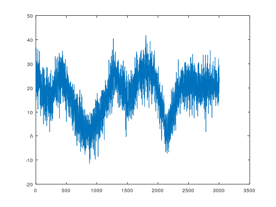
n = 300

isi = round(exp(randn(n,1))*10);

spike_ts = 0;
for i=1:n
    spike_ts(length(spike_ts)+isi(i))=1;
end
figure(++fignums), clf
plot(spike_ts)
n = 300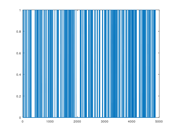
atk
mtk
atk = notebookmtk = plotlygraphics_toolkit(atk)
set(gcf,'Visible','on')
hist(isi, 30);
graphics_toolkit(atk);
figure(10), clf
hist(isi, 30);
set(gcf,'Visible','on')
graphics_toolkit(toolkit);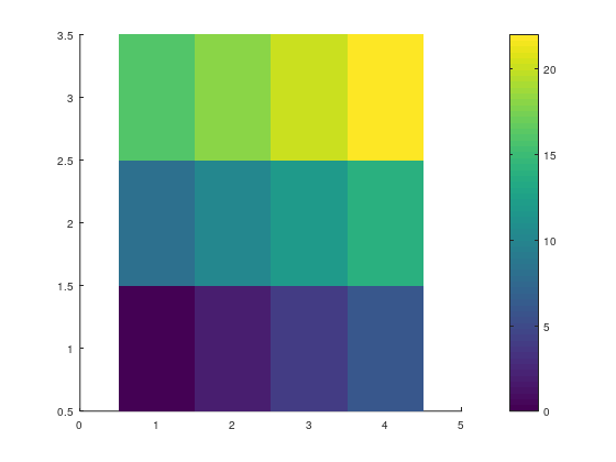
help randn'randn' is a built-in function from the file libinterp/corefcn/rand.cc
-- randn (N)
-- randn (M, N, ...)
-- randn ([M N ...])
-- V = randn ("state")
-- randn ("state", V)
-- randn ("state", "reset")
-- V = randn ("seed")
-- randn ("seed", V)
-- randn ("seed", "reset")
-- randn (..., "single")
-- randn (..., "double")
Return a matrix with normally distributed random elements having
zero mean and variance one.
The arguments are handled the same as the arguments for ‘rand’.
By default, ‘randn’ uses the Marsaglia and Tsang “Ziggurat
technique” to transform from a uniform to a normal distribution.
The class of the value returned can be controlled by a trailing
"double" or "single" argument. These are the only valid classes.
Reference: G. Marsaglia and W.W. Tsang, ‘Ziggurat Method for
Generating Random Variables’, J. Statistical Software, vol 5, 2000,
<https://www.jstatsoft.org/v05/i08/>
See also: rand, rande, randg, randp.
Additional help for built-in functions and operators is
available in the online version of the manual. Use the command
'doc <topic>' to search the manual index.
Help and information about Octave is also available on the WWW
at https://www.octave.org and via the help@octave.org
mailing list.n = 2000
figure(++fignums), clf
randn('seed', 420)
plot(cumsum(randn(n,1)))n = 2000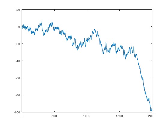
\[ y_t = \frac{1}{2k+1}\sum_{i=t-k}^{t+k}x_i \]
function filtsig = filter_mean(signal, k=20, initzeros=true)
    if initzeros
        filtsig = zeros(size(signal));
    else
        filtsig = signal;
    end
    n = length(signal);
    for i=k+1:n-k-1
        filtsig(i) = mean(signal(i-k:i+k));
    end
endfunction
signal = random_signal();
filtsig = filter_mean(signal, k=20, initzeros=false);
filtsig;windowsize = 1000*(k*2+1)/sratewindowsize = 41help dsearchn'dsearchn' is a function from the file /home/rahuketu/anaconda3/envs/octave/share/octave/7.2.0/m/geometry/dsearchn.m
-- IDX = dsearchn (X, TRI, XI)
-- IDX = dsearchn (X, TRI, XI, OUTVAL)
-- IDX = dsearchn (X, XI)
-- [IDX, D] = dsearchn (...)
Return the index IDX of the closest point in X to the elements XI.
If OUTVAL is supplied, then the values of XI that are not contained
within one of the simplices TRI are set to OUTVAL. Generally, TRI
is returned from ‘delaunayn (X)’.
The optional output D contains a column vector of distances between
the query points XI and the nearest simplex points X.
See also: dsearch, tsearch.
Additional help for built-in functions and operators is
available in the online version of the manual. Use the command
'doc <topic>' to search the manual index.
Help and information about Octave is also available on the WWW
at https://www.octave.org and via the help@octave.org
mailing list.figure(++fignums), clf, hold on
plot(time, signal, time, filtsig, 'linewidth', 2)
tidx = dsearchn(time',1);
ylim = get(gca,'ylim');
patch(time([ tidx-k tidx-k tidx+k tidx+k ]),ylim([ 1 2 2 1 ]),'k','facealpha',.25,'linestyle','none');
plot(time([tidx tidx]),ylim,'k');
xlabel('Time (sec.)'), ylabel('Amplitude');
title([ 'Running-mean filter with a k=' num2str(round(windowsize)) '-ms filter' ]);
legend({'Signal';'Filtered';'Window';'window center'});
zoom on
tidx = dsearchn(time', 1); tidxtidx = 1001help patch'patch' is a function from the file /home/rahuketu/anaconda3/envs/octave/share/octave/7.2.0/m/plot/draw/patch.m
-- patch ()
-- patch (X, Y, C)
-- patch (X, Y, Z, C)
-- patch ("Faces", FACES, "Vertices", VERTS, ...)
-- patch (..., PROP, VAL, ...)
-- patch (..., PROPSTRUCT, ...)
-- patch (HAX, ...)
-- H = patch (...)
Create patch object in the current axes with vertices at locations
(X, Y) and of color C.
If the vertices are matrices of size MxN then each polygon patch
has M vertices and a total of N polygons will be created. If some
polygons do not have M vertices use NaN to represent "no vertex".
If the Z input is present then 3-D patches will be created.
The color argument C can take many forms. To create polygons which
all share a single color use a string value (e.g., "r" for red), a
scalar value which is scaled by ‘caxis’ and indexed into the
current colormap, or a 3-element RGB vector with the precise
TrueColor.
If C is a vector of length N then the ith polygon will have a color
determined by scaling entry C(i) according to ‘caxis’ and then
indexing into the current colormap. More complicated coloring
situations require directly manipulating patch property/value
pairs.
Instead of specifying polygons by matrices X and Y, it is possible
to present a unique list of vertices and then a list of polygon
faces created from those vertices. In this case the "Vertices"
matrix will be an Nx2 (2-D patch) or Nx3 (3-D patch). The MxN
"Faces" matrix describes M polygons having N vertices—each row
describes a single polygon and each column entry is an index into
the "Vertices" matrix to identify a vertex. The patch object can
be created by directly passing the property/value pairs
"Vertices"/VERTS, "Faces"/FACES as inputs.
Instead of using property/value pairs, any property can be set by
passing a structure PROPSTRUCT with the respective field names.
If the first argument HAX is an axes handle, then plot into this
axes, rather than the current axes returned by ‘gca’.
The optional return value H is a graphics handle to the created
patch object.
Programming Note: The full list of properties is documented at
Patch Properties. Useful patch properties include: "cdata",
"edgecolor", "facecolor", "faces", and "facevertexcdata".
See also: fill, get, set.
Additional help for built-in functions and operators is
available in the online version of the manual. Use the command
'doc <topic>' to search the manual index.
Help and information about Octave is also available on the WWW
at https://www.octave.org and via the help@octave.org
mailing list.A = [ 1 2; 2 1]| A | 1 | 2 |
| 1 | 1 | 2 |
| 2 | 2 | 1 |
graphics_toolkit(atk)
figure(++fignums), clf, hold on
C = [0 2 4 6; 8 10 12 14; 16 18 20 22];
imagesc(C)
colorbar
graphics_toolkit(toolkit)
k = 20
ones(1, 2*k+1)/(2*k+1)
k = 20| ans | 1 | 2 | 3 | 4 | 5 | 6 | 7 | 8 | 9 | 10 | 11 | 12 | 13 | 14 | 15 | 16 | 17 | 18 | 19 | 20 | 21 | 22 | 23 | 24 | 25 | 26 | 27 | 28 | 29 | 30 | 31 | 32 | 33 | 34 | 35 | 36 | 37 | 38 | 39 | 40 | 41 |
| 1 | 0.0243902 | 0.0243902 | 0.0243902 | 0.0243902 | 0.0243902 | 0.0243902 | 0.0243902 | 0.0243902 | 0.0243902 | 0.0243902 | 0.0243902 | 0.0243902 | 0.0243902 | 0.0243902 | 0.0243902 | 0.0243902 | 0.0243902 | 0.0243902 | 0.0243902 | 0.0243902 | 0.0243902 | 0.0243902 | 0.0243902 | 0.0243902 | 0.0243902 | 0.0243902 | 0.0243902 | 0.0243902 | 0.0243902 | 0.0243902 | 0.0243902 | 0.0243902 | 0.0243902 | 0.0243902 | 0.0243902 | 0.0243902 | 0.0243902 | 0.0243902 | 0.0243902 | 0.0243902 | 0.0243902 |
function g = uniform(k, normalize=false)
    g = ones(1, 2*k+1);
    if normalize
        g = g/sum(g);
    end
endfunctionuniform(k=20)| ans | 1 | 2 | 3 | 4 | 5 | 6 | 7 | 8 | 9 | 10 | 11 | 12 | 13 | 14 | 15 | 16 | 17 | 18 | 19 | 20 | 21 | 22 | 23 | 24 | 25 | 26 | 27 | 28 | 29 | 30 | 31 | 32 | 33 | 34 | 35 | 36 | 37 | 38 | 39 | 40 | 41 |
| 1 | 1 | 1 | 1 | 1 | 1 | 1 | 1 | 1 | 1 | 1 | 1 | 1 | 1 | 1 | 1 | 1 | 1 | 1 | 1 | 1 | 1 | 1 | 1 | 1 | 1 | 1 | 1 | 1 | 1 | 1 | 1 | 1 | 1 | 1 | 1 | 1 | 1 | 1 | 1 | 1 | 1 |
\[ y_t = \sum_{i=t-k}^{t+k}x_ig_i \]
where g is
\[ g = e^{\frac{-4 ln(2) t^2}{w^2}} \]
w = Full width half minimum(width at 0.5 gain)
Notes - Gaussian smoothes out edges even more than mean filter
log(2), exp(2)
t = linspace(1, 2,  5)
w = 2
-4*log(2)*t.^2/ w^2
ans = 0.6931ans = 7.3891| t | 1 | 2 | 3 | 4 | 5 |
| 1 | 1 | 1.25 | 1.5 | 1.75 | 2 |
w = 2| ans | 1 | 2 | 3 | 4 | 5 |
| 1 | -0.693147 | -1.08304 | -1.55958 | -2.12276 | -2.77259 |
function g = gaussian(t, w, normalize=false)
    g = exp( -4*log(2)*t.^2/w^2);
    if normalize
        g = g/sum(g)
    end
endfunction
t = linspace(-4, 4, 50);
figure(++fignums), clf
plot(gaussian(t,w=2))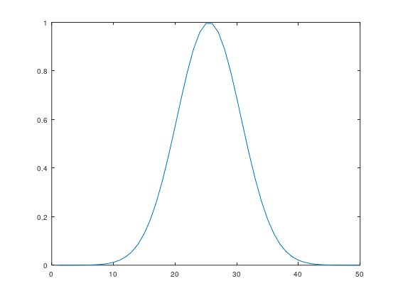
srate = 1000;
fwhm = 25.5483213524
k = 50;
gtime = 1000*(-k:k)/srate;
gaus_win = gaussian(gtime, fwhm);
pre_peak_half = k + dsearchn(gaus_win(k+1:end)', 0.5)
post_peak_half = dsearchn(gaus_win(1:k)', 0.5)

exp_fwhm = gtime(pre_peak_half) - gtime(post_peak_half)
fwhm = 25.548pre_peak_half = 64post_peak_half = 38exp_fwhm = 26figure(++fignums), clf, hold on
plot(gtime, gaus_win, 'ko-', 'markerfacecolor', 'w', 'linewidth', 2)
plot(gtime([pre_peak_half post_peak_half]),gaus_win([pre_peak_half post_peak_half]),'m','linewidth',3)
gaus_win = gaus_win / sum(gaus_win);
title([ 'Gaussian kernel with requeted FWHM ' num2str(fwhm) ' ms (' num2str(exp_fwhm) ' ms achieved)' ])
xlabel('Time (ms)'), ylabel('Gain')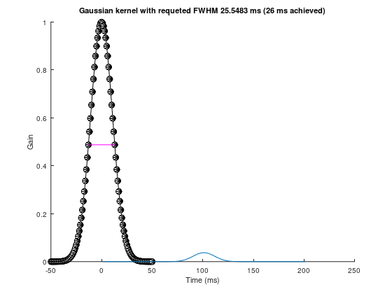
function filtsig = apply_filter(signal, filter_pdf, k=20, initzeros=true)
    if initzeros
        filtsig = zeros(size(signal));
    else
        filtsig = signal;
    end
    n = length(signal);
    for i=k+1:n-k-1
        filtsig(i) = sum(signal(i-k:i+k).*filter_pdf);
    end
endfunctionsrate = 1000;
fwhm = 25.5483213524
k = 40;
gtime = 1000*(-k:k)/srate;
gaus_win = gaussian(gtime, fwhm, normalize=true);
uniform_win = uniform(k, normalize=true);
filtsig_uniform = apply_filter(signal, uniform_win, k=k, initzeros=false);
filtsig_gaussian = apply_filter(signal, gaus_win, k=k, initzeros=false);fwhm = 25.548| g | 1 | 2 | 3 | 4 | 5 | 6 | 7 | 8 | 9 | 10 | 11 | 12 | 13 | 14 | 15 | 16 | 17 | 18 | 19 | 20 | 21 | 22 | 23 | 24 | 25 | 26 | 27 | 28 | 29 | 30 | 31 | 32 | 33 | 34 | 35 | 36 | 37 | 38 | 39 | 40 | 41 | 42 | 43 | 44 | 45 | 46 | 47 | 48 | 49 | 50 | 51 | 52 | 53 | 54 | 55 | 56 | 57 | 58 | 59 | 60 | 61 | 62 | 63 | 64 | 65 | 66 | 67 | 68 | 69 | 70 | 71 | 72 | 73 | 74 | 75 | 76 | 77 | 78 | 79 | 80 | 81 |
| 1 | 4.11089e-05 | 5.75008e-05 | 7.97484e-05 | 0.000109668 | 0.000149537 | 0.000202176 | 0.000271031 | 0.000360263 | 0.000474822 | 0.000620514 | 0.000804051 | 0.00103306 | 0.00131607 | 0.00166242 | 0.00208216 | 0.00258582 | 0.00318414 | 0.00388774 | 0.00470666 | 0.00564987 | 0.00672472 | 0.00793635 | 0.00928705 | 0.0107757 | 0.0123972 | 0.014142 | 0.0159959 | 0.0179399 | 0.0199498 | 0.0219973 | 0.0240497 | 0.0260711 | 0.0280234 | 0.0298671 | 0.0315628 | 0.0330725 | 0.0343614 | 0.0353984 | 0.0361583 | 0.036622 | 0.0367779 | 0.036622 | 0.0361583 | 0.0353984 | 0.0343614 | 0.0330725 | 0.0315628 | 0.0298671 | 0.0280234 | 0.0260711 | 0.0240497 | 0.0219973 | 0.0199498 | 0.0179399 | 0.0159959 | 0.014142 | 0.0123972 | 0.0107757 | 0.00928705 | 0.00793635 | 0.00672472 | 0.00564987 | 0.00470666 | 0.00388774 | 0.00318414 | 0.00258582 | 0.00208216 | 0.00166242 | 0.00131607 | 0.00103306 | 0.000804051 | 0.000620514 | 0.000474822 | 0.000360263 | 0.000271031 | 0.000202176 | 0.000149537 | 0.000109668 | 7.97484e-05 | 5.75008e-05 | 4.11089e-05 |
figure(++fignums), clf, hold on
plot(time, signal, time, filtsig_uniform,'m','linewidth', 2, time, filtsig_gaussian,'g', 'linewidth', 2)
legend('signal', 'mean', 'gaussian')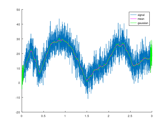
fwhm = 25
k = 100;
gtime = -k:k;
gaus_win2 = gaussian(gtime, fwhm, normalize=true);
filtsig_spike = apply_filter(spike_ts, gaus_win2, k=k, initzeros=true);
figure(12)
plot(gaus_win2)
fwhm = 25| g | 1 | 2 | 3 | 4 | 5 | 6 | 7 | 8 | 9 | 10 | 11 | 12 | 13 | 14 | 15 | 16 | 17 | 18 | 19 | 20 | 21 | 22 | 23 | 24 | 25 | 26 | 27 | 28 | 29 | 30 | 31 | 32 | 33 | 34 | 35 | 36 | 37 | 38 | 39 | 40 | 41 | 42 | 43 | 44 | 45 | 46 | 47 | 48 | 49 | 50 | 51 | 52 | 53 | 54 | 55 | 56 | 57 | 58 | 59 | 60 | 61 | 62 | 63 | 64 | 65 | 66 | 67 | 68 | 69 | 70 | 71 | 72 | 73 | 74 | 75 | 76 | 77 | 78 | 79 | 80 | 81 | 82 | 83 | 84 | 85 | 86 | 87 | 88 | 89 | 90 | 91 | 92 | 93 | 94 | 95 | 96 | 97 | 98 | 99 | 100 | 101 | 102 | 103 | 104 | 105 | 106 | 107 | 108 | 109 | 110 | 111 | 112 | 113 | 114 | 115 | 116 | 117 | 118 | 119 | 120 | 121 | 122 | 123 | 124 | 125 | 126 | 127 | 128 | 129 | 130 | 131 | 132 | 133 | 134 | 135 | 136 | 137 | 138 | 139 | 140 | 141 | 142 | 143 | 144 | 145 | 146 | 147 | 148 | 149 | 150 | 151 | 152 | 153 | 154 | 155 | 156 | 157 | 158 | 159 | 160 | 161 | 162 | 163 | 164 | 165 | 166 | 167 | 168 | 169 | 170 | 171 | 172 | 173 | 174 | 175 | 176 | 177 | 178 | 179 | 180 | 181 | 182 | 183 | 184 | 185 | 186 | 187 | 188 | 189 | 190 | 191 | 192 | 193 | 194 | 195 | 196 | 197 | 198 | 199 | 200 | 201 |
| 1 | 2.03708e-21 | 4.92493e-21 | 1.18015e-20 | 2.80301e-20 | 6.59867e-20 | 1.5397e-19 | 3.56091e-19 | 8.1627e-19 | 1.85461e-18 | 4.17657e-18 | 9.32251e-18 | 2.06249e-17 | 4.52272e-17 | 9.82999e-17 | 2.11765e-16 | 4.52169e-16 | 9.56962e-16 | 2.00741e-15 | 4.17372e-15 | 8.60118e-15 | 1.75687e-14 | 3.55686e-14 | 7.13744e-14 | 1.41959e-13 | 2.79855e-13 | 5.46824e-13 | 1.05903e-12 | 2.03291e-12 | 3.8679e-12 | 7.2942e-12 | 1.36341e-11 | 2.52594e-11 | 4.63838e-11 | 8.44222e-11 | 1.52298e-10 | 2.72318e-10 | 4.82622e-10 | 8.47782e-10 | 1.47607e-09 | 2.54729e-09 | 4.35709e-09 | 7.38688e-09 | 1.24129e-08 | 2.06743e-08 | 3.41299e-08 | 5.58454e-08 | 9.05703e-08 | 1.4559e-07 | 2.31965e-07 | 3.66321e-07 | 5.73387e-07 | 8.89571e-07 | 1.36792e-06 | 2.0849e-06 | 3.14963e-06 | 4.71606e-06 | 6.99916e-06 | 1.02958e-05 | 1.50113e-05 | 2.16934e-05 | 3.10728e-05 | 4.41145e-05 | 6.20768e-05 | 8.65812e-05 | 0.000119692 | 0.000164003 | 0.000222734 | 0.000299826 | 0.000400035 | 0.000529021 | 0.000693418 | 0.000900874 | 0.00116006 | 0.00148062 | 0.00187306 | 0.00234859 | 0.00291884 | 0.00359551 | 0.00438993 | 0.00531252 | 0.00637222 | 0.00757579 | 0.00892713 | 0.0104266 | 0.0120704 | 0.0138498 | 0.0157513 | 0.0177555 | 0.019838 | 0.021969 | 0.024114 | 0.0262346 | 0.0282895 | 0.030236 | 0.032031 | 0.0336328 | 0.0350028 | 0.0361068 | 0.0369166 | 0.0374112 | 0.0375775 | 0.0374112 | 0.0369166 | 0.0361068 | 0.0350028 | 0.0336328 | 0.032031 | 0.030236 | 0.0282895 | 0.0262346 | 0.024114 | 0.021969 | 0.019838 | 0.0177555 | 0.0157513 | 0.0138498 | 0.0120704 | 0.0104266 | 0.00892713 | 0.00757579 | 0.00637222 | 0.00531252 | 0.00438993 | 0.00359551 | 0.00291884 | 0.00234859 | 0.00187306 | 0.00148062 | 0.00116006 | 0.000900874 | 0.000693418 | 0.000529021 | 0.000400035 | 0.000299826 | 0.000222734 | 0.000164003 | 0.000119692 | 8.65812e-05 | 6.20768e-05 | 4.41145e-05 | 3.10728e-05 | 2.16934e-05 | 1.50113e-05 | 1.02958e-05 | 6.99916e-06 | 4.71606e-06 | 3.14963e-06 | 2.0849e-06 | 1.36792e-06 | 8.89571e-07 | 5.73387e-07 | 3.66321e-07 | 2.31965e-07 | 1.4559e-07 | 9.05703e-08 | 5.58454e-08 | 3.41299e-08 | 2.06743e-08 | 1.24129e-08 | 7.38688e-09 | 4.35709e-09 | 2.54729e-09 | 1.47607e-09 | 8.47782e-10 | 4.82622e-10 | 2.72318e-10 | 1.52298e-10 | 8.44222e-11 | 4.63838e-11 | 2.52594e-11 | 1.36341e-11 | 7.2942e-12 | 3.8679e-12 | 2.03291e-12 | 1.05903e-12 | 5.46824e-13 | 2.79855e-13 | 1.41959e-13 | 7.13744e-14 | 3.55686e-14 | 1.75687e-14 | 8.60118e-15 | 4.17372e-15 | 2.00741e-15 | 9.56962e-16 | 4.52169e-16 | 2.11765e-16 | 9.82999e-17 | 4.52272e-17 | 2.06249e-17 | 9.32251e-18 | 4.17657e-18 | 1.85461e-18 | 8.1627e-19 | 3.56091e-19 | 1.5397e-19 | 6.59867e-20 | 2.80301e-20 | 1.18015e-20 | 4.92493e-21 | 2.03708e-21 |

figure(++fignums), clf, hold on
plot(spike_ts)
plot(filtsig_spike, 'linewidth', 2)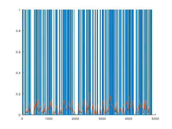
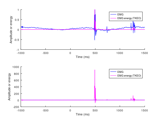
\[ y_t = x_t^2 - x_{t-1}x_{t+1} \]
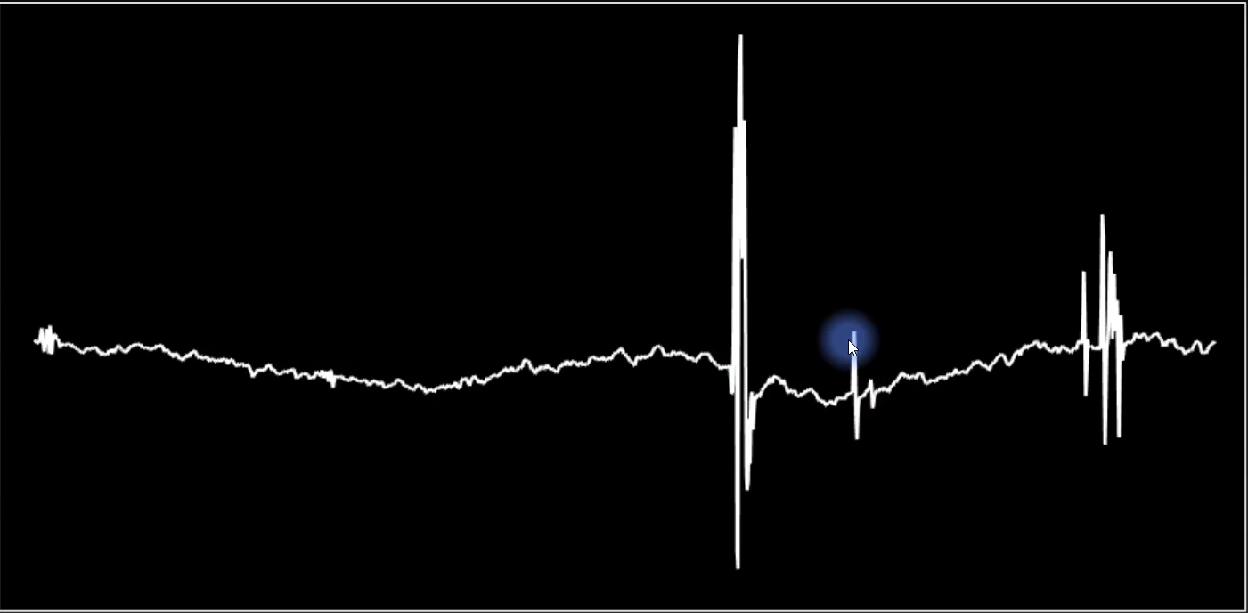
load(fullfile(cd, "resources","section_02","emg4TKEO.mat" )); whosVariables visible from the current scope:
variables in scope: top scope
Attr Name Size Bytes Class
==== ==== ==== ===== =====
A 2x2 32 double
C 3x4 96 double
a 1x2 16 double
ampl 1x3001 24008 double
ans 1x1 8 double
atk 1x8 8 char
doc_file 1x79 79 char
emg 1x1281 5124 single
emgtime 1x1281 10248 double
exp_fwhm 1x1 8 double
fignums 1x1 8 double
filtsig 1x3001 24008 double
filtsig_gaussian 1x3001 24008 double
filtsig_spike 1x4858 38864 double
filtsig_uniform 1x3001 24008 double
fs 1x1 8 double
fwhm 1x1 8 double
gaus_win 1x81 648 double
gaus_win2 1x201 1608 double
gtime 1x201 24 double
i 1x1 8 double
initzeros 1x1 1 logical
isi 300x1 2400 double
k 1x1 8 double
mtk 1x6 6 char
n 1x1 8 double
noise 1x3001 24008 double
noiseamp 1x1 8 double
normalize 1x1 1 logical
p 1x1 8 double
pkg_dir 1x64 64 char
post_peak_half 1x1 8 double
pre_peak_half 1x1 8 double
s 1x2 16 double
signal 1x3001 24008 double
spike_ts 1x4858 38864 double
srate 1x1 8 double
t 1x50 400 double
tidx 1x1 8 double
time 1x3001 24 double
toolkit 1x8 8 char
uniform_win 1x81 648 double
w 1x1 8 double
windowsize 1x1 8 double
ylim 1x2 16 double
Total is 34404 elements using 243371 bytes
figure(++fignums), clf, hold on
plot(emgtime, emg)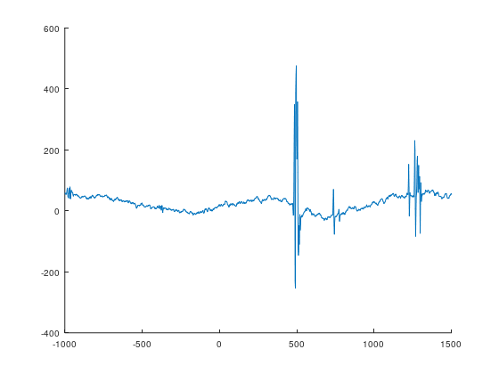
function tkeo = apply_tkeo(signal)
    tkeo = signal;
    for i=2:length(signal)-1
        tkeo(i) = signal(i)^2 - signal(i-1)*signal(i+1);
    end
endfunction
function tkeo = apply_tkeo_vec(signal)
tkeo = signal;
tkeo(2:end-1) = signal(2:end-1).^2 - signal(1: end-2).*signal(3:end);
endfunctionfigure(++fignums), clf, hold on
plot(emgtime, emg)
plot(emgtime, apply_tkeo(emg))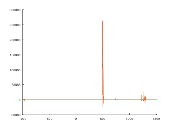
function signalz = to_zscore(signal, signaltime, time_cutoff=0)
    time0 = dsearchn(signaltime', time_cutoff);
    signalz = (signal - mean(signaltime(1:time0)))/ std(signaltime(1:time0));
endfunctionfigure(++fignums), clf
tkeo = apply_tkeo_vec(emg);
subplot(211), hold on
plot(emgtime, emg./max(emg), 'b', 'linewidth', 2)
plot(emgtime, tkeo./max(tkeo), 'm', 'linewidth', 2)
xlabel('Time (ms)'), ylabel('Amplitude or energy')
legend("EMG", "EMG energy (TKEO)")
subplot(212), hold on
plot(emgtime, to_zscore(emg, emgtime, time_cutoff=0), 'b', 'linewidth', 2)
plot(emgtime, to_zscore(tkeo, emgtime, time_cutoff=0), 'm', 'linewidth', 2)
xlabel('Time (ms)'), ylabel('Amplitude or energy')
legend("EMG", "EMG energy (TKEO)")