import sklearn1-D Partial Dependence Plots
Important
- How a feature/variable affect our predictions?
- Calculated after model has been fit
Example questions
Controlling for all other house features, what impact do longitude and latitude have on home prices? To restate this, how would similarly sized houses be priced in different areas?
Are predicted health differences between two groups due to differences in their diets, or due to some other factor?
Also
- For linear or logistic regression models, partial dependence plots can be interpreted similarly to the coefficients in those models. Though, partial dependence plots on sophisticated models can capture more complex patterns than coefficients from simple models
sklearn.__version__'1.5.0'from aiking.data.external import *
import numpy as np
import pandas as pd
from sklearn.model_selection import train_test_split
from sklearn.ensemble import RandomForestClassifier
from sklearn.tree import DecisionTreeClassifier, plot_tree
from sklearn.inspection import PartialDependenceDisplay
import seaborn as sns
import matplotlib.pyplot as plt
import pdpbox
import graphviz
import panel as pn
from ipywidgets import interact
import pdpboxpn.extension('plotly')path = get_ds('fifa-2018-match-statistics'); path.ls()[0]Path('/Users/rahul1.saraf/rahuketu/programming/AIKING_HOME/data/fifa-2018-match-statistics/FIFA 2018 Statistics.csv')df = pd.read_csv(path/"FIFA 2018 Statistics.csv"); df
y = (df['Man of the Match'] == "Yes"); y
X = df.select_dtypes(np.int64); X
df_train, df_val, y_train, y_val = train_test_split(X, y, random_state=1)
df_train.shape, df_val.shape, y_train.shape, y_val.shape((96, 18), (32, 18), (96,), (32,))model_dt = DecisionTreeClassifier(random_state=0, max_depth=5, min_samples_split=5).fit(df_train, y_train); model_dtDecisionTreeClassifier(max_depth=5, min_samples_split=5, random_state=0)In a Jupyter environment, please rerun this cell to show the HTML representation or trust the notebook.
On GitHub, the HTML representation is unable to render, please try loading this page with nbviewer.org.
DecisionTreeClassifier(max_depth=5, min_samples_split=5, random_state=0)
fig, ax = plt.subplots(1, figsize= (15, 15))
plot_tree(model_dt,filled=True,feature_names=df_train.columns.tolist(),fontsize=10,ax=ax);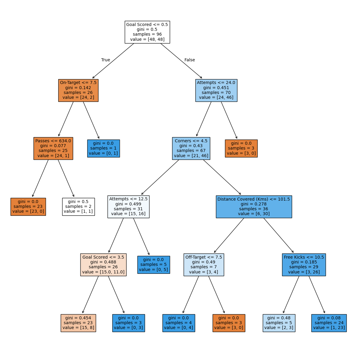
Partial plot presents the changes from what would be predicted at baseline or left most value
PartialDependenceDisplay.from_estimator(model_dt, df_val, ['Goal Scored', 'On-Target'])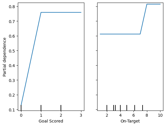
PartialDependenceDisplay.from_estimator(model_dt, df_val, ['Distance Covered (Kms)'])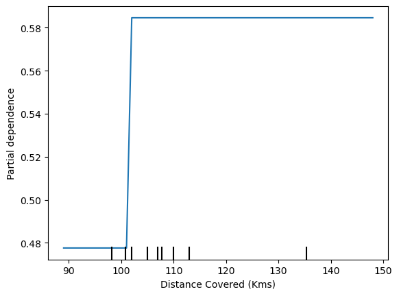
df_train.columns.tolist()['Goal Scored',
'Ball Possession %',
'Attempts',
'On-Target',
'Off-Target',
'Blocked',
'Corners',
'Offsides',
'Free Kicks',
'Saves',
'Pass Accuracy %',
'Passes',
'Distance Covered (Kms)',
'Fouls Committed',
'Yellow Card',
'Yellow & Red',
'Red',
'Goals in PSO']feature = df_train.columns.tolist()[0]
PartialDependenceDisplay.from_estimator(model_dt, df_val, [feature]);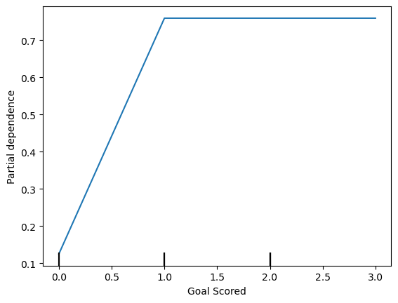
feature = df_train.columns.tolist()[0]
PartialDependenceDisplay.from_estimator(model_dt, df_val, [feature], kind='both');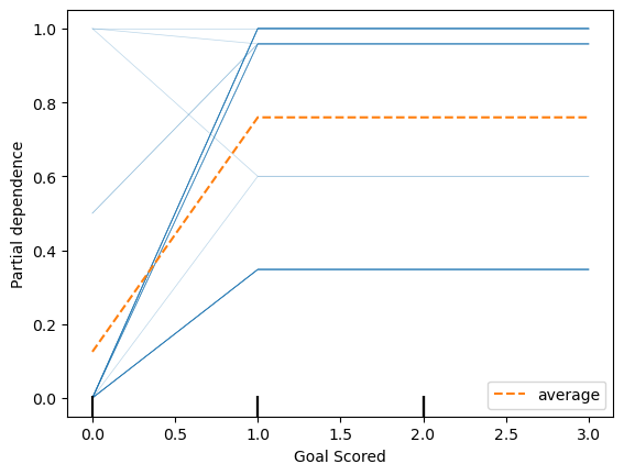
model_rf = RandomForestClassifier(random_state=0).fit(df_train, y_train); model_rfRandomForestClassifier(random_state=0)In a Jupyter environment, please rerun this cell to show the HTML representation or trust the notebook.
On GitHub, the HTML representation is unable to render, please try loading this page with nbviewer.org.
RandomForestClassifier(random_state=0)
feature = df_train.columns.tolist()[0]
PartialDependenceDisplay.from_estimator(model_rf, df_val, [feature], kind='both');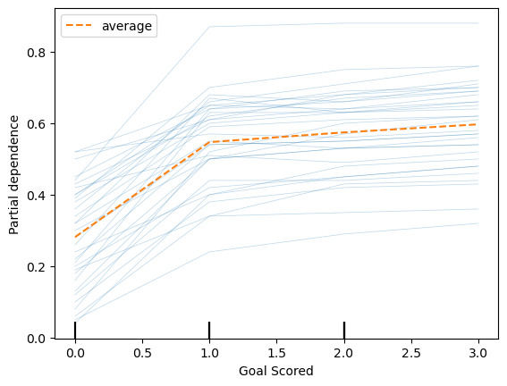
feature = 'Distance Covered (Kms)'
PartialDependenceDisplay.from_estimator(model_rf, df_val, [feature], kind='both');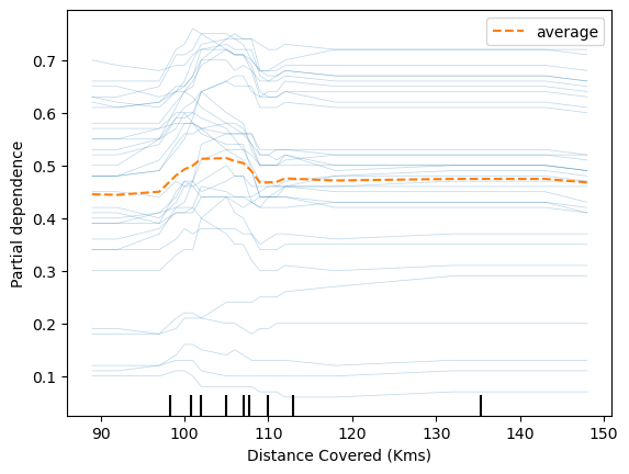
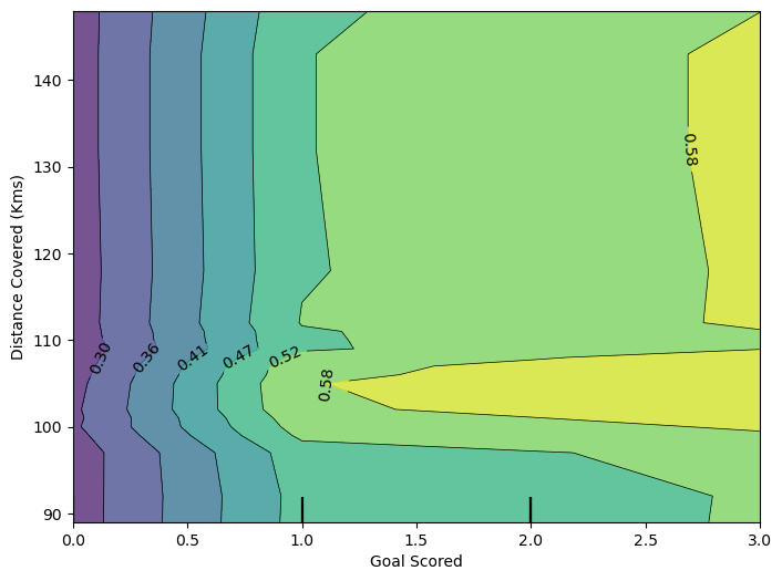
fig, ax = plt.subplots(figsize=(8, 6))
features = [('Goal Scored', 'Distance Covered (Kms)')]

PartialDependenceDisplay.from_estimator(model_dt, df_val, features, ax=ax);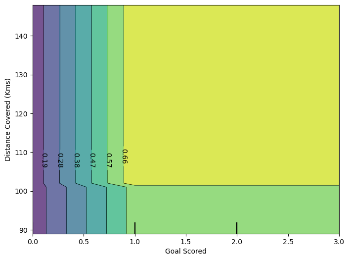
fig, ax = plt.subplots(figsize=(8, 6))
features = [('Goal Scored', 'Distance Covered (Kms)')]

PartialDependenceDisplay.from_estimator(model_rf, df_val, features, ax=ax);