Risk Management under Volatility Clustering

Introduction

Here are a few things covered during this week.

• What is the objective of risk management?
  • To create a statistical model for future returns , in particular the left tail.
  • Model if often based on historical returns ( the only thing that we can observe)
  • Future Distribution of Returns(TR) = Function (Historical Returns , Some assumptions)
• Modelling assumptions so far
  • Future Distribution ( WILSHIRE 5000/ index fund) == Historical Distribution ( True for some time but not always)
    • Currently our distribution of choice is re-scaled T-distribution as it models the data better than normal distribution .
    • We have also simulated observed distribution from the data
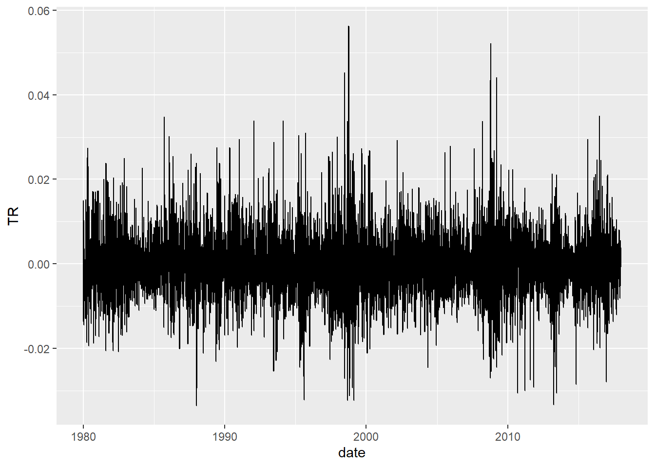
  • Parameters of historical distribution ( mean, sigma and/ or df) are calculated without paying attention to the ordering of the data
    • Implies, even if we randomly permeates logret series distribution parameter will still be same.
• What if we have some information in the past which can inform us about the future distribution for logret? In other words, what is the impact of serial correlation if any.
• Serial correlation
  • Positive serial correlation - an above average return ( > mean) tend to be followed by another above - average return
  • Negative serial correlation - above average return is followed by below average return
  • No correlation / random wal k - an above average return does not increase the likelihood of being followed by an above avg or below avg return.
  • There was a long history of research in financial markets that look at serial correlation. Now to understand what serial correlation means,
  • Correlation - let’s start with the correlation between two variables, let’s say, X and Y. The correlation coefficient between X and Y measures how they co-move together. We say that X and Y are positively correlated when they tend to move up and down together. To be more precise, if X is above its mean, then Y is likely to be also above its mean.
  • Serial correlation - How a variable X and its own past are correlated?
• Significance of serial correlation in Finance is associated with the concept of Market Efficiency.

  • The theory of market efficiency says that the observed price of an asset such as a stock, fully reflects all information about that asset

  • When new information comes in, it will change the price of the asset. Good news presumably will lead to an increase in its price. Conversely, bad news will lead to a decrease in its price.

  • Now, because all existing information has been incorporated in the price of an asset, any new information must be a surprise.

  • If the surprise is good news, the price of the asset will go up, and if the surprise is bad news, the price of the asset will go down. But there is no way to tell ahead of time whether the news is good or bad. So there is no way to tell if the price will go up or down.

  • This is so called random walk model of prices.

  • This random walk model just says there is no way to predict if the future price of an asset will go up or go down relative to its current price.

  • An implication of the random walk model is that returns have no serial correlation. So testing for serial correlation in stock return has been viewed as testing for market efficiency

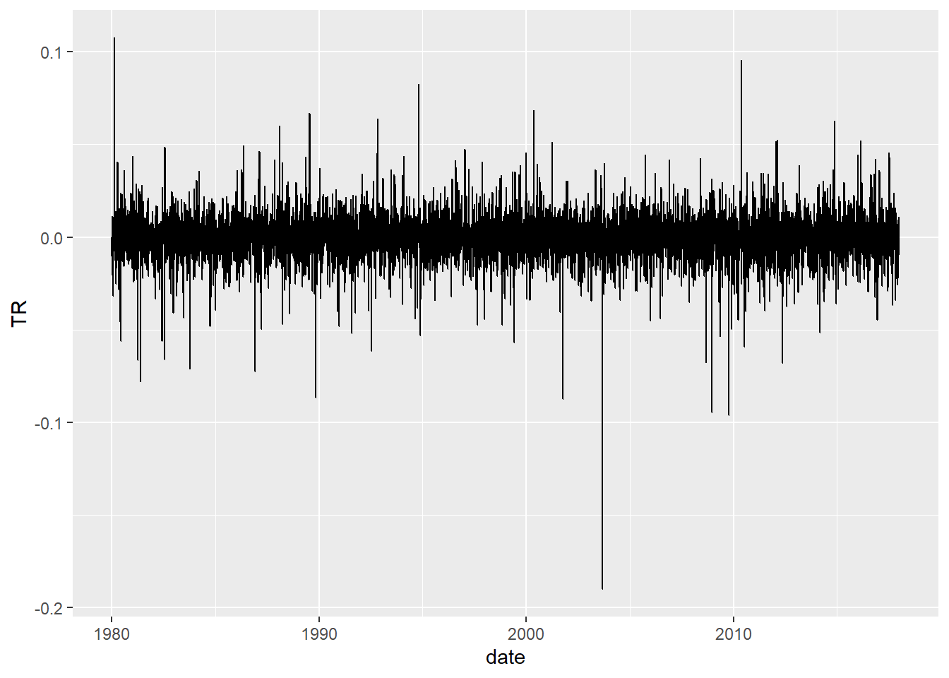
• Motivation & Definition for Volatility Clustering - In financial time series data, it is often observed

  • Large returns +ve/ -ve negative tend to be followed by more large returns

    • High Volatility days are followed by more High Volatility days

    • Low Volatility days are followed by more Low Volatility days

  • This phenomenon is called Volatility clustering

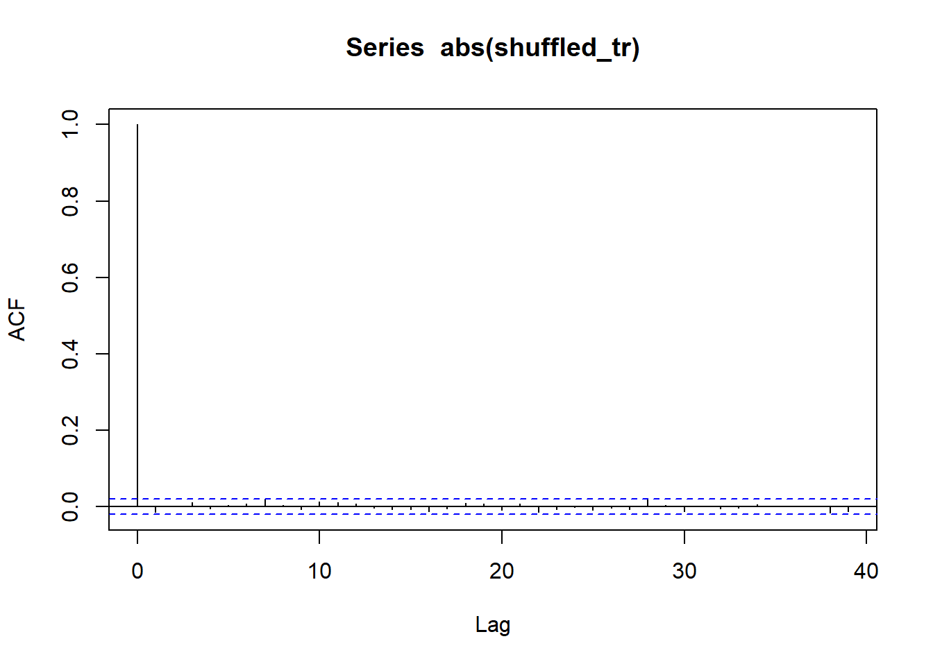
  • It is calculated mathematically by measuring autocorrelation of absolute values of log returns

  • A time series exhibiting Volatility clustering implies ordering of the data is important

  • Strong volatility clustering implies we can predict volatility of stock prices for future values based on the past values.

  • This is exploited in GARCH model ( Generalized Auto-regressive Conditional Heteroskedasticity)

  • We can test volatility clustering/ effect of ordering by

    • Plotting acf on absolute values of logreturns - ( Should show strong evidence of serial correlation )

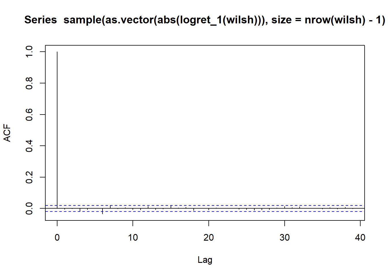
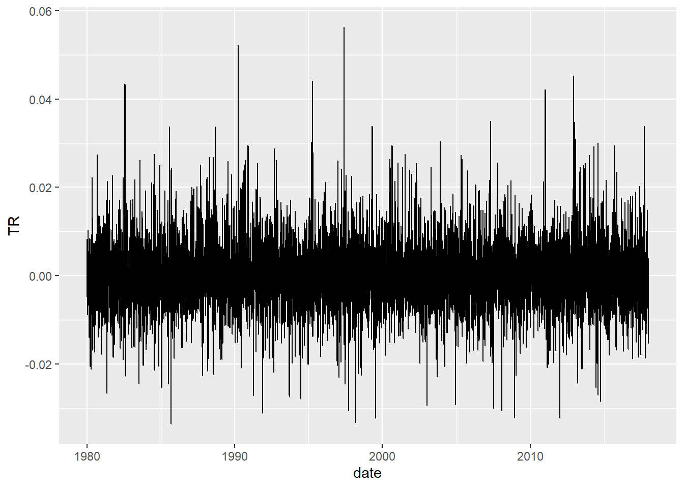
    • Shuffling/ Permeating returns and apply same logic again ( Should show no evidence of serial correlation on shuffled series)

• GARCH model
  • WILSHIRE 5000 ACF plot indicates no/ weak evidence of serial correlation => Difficult to predict mean of future values based on historical values
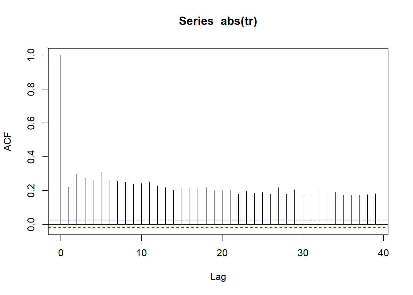
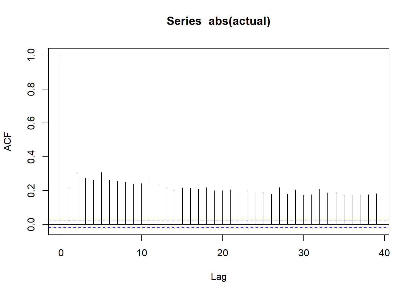
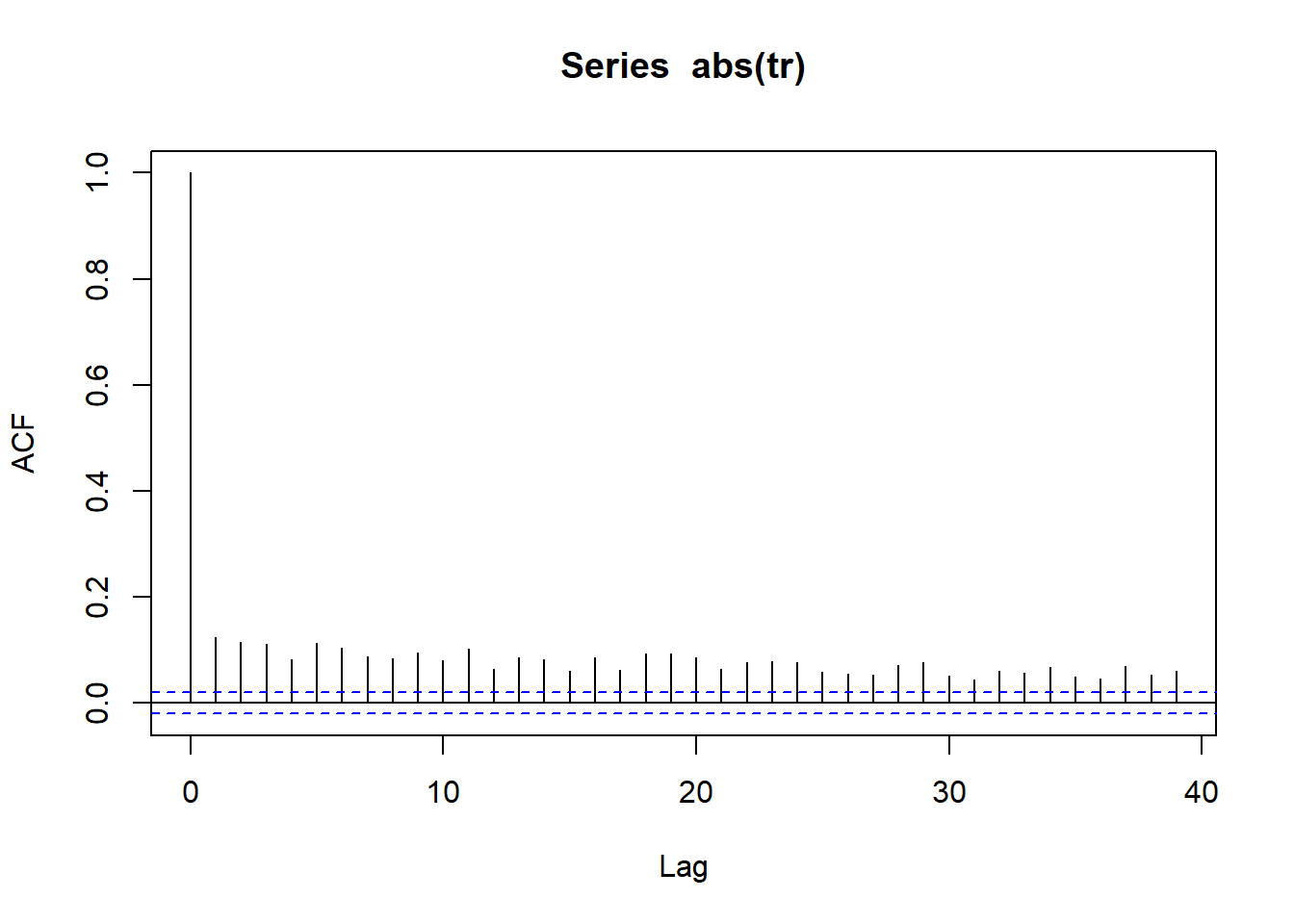
  • WILSHIRE 5000 ABS(ACF) plot indicates strong volatility clustering =>Volatility / Standard Deviation is changing over time in a predictable manner.
  • What we want is a statistical model which allows us to predict future volatility- GARCH
  • GARCH model has many extensions. We are going to focus on GARCH(1,1). It is one of the simplest GARCH model .But it does a very good job on WILSHIRE 5000 data in modelling volatility clustering.
  • GARCH(1,1)-normal model is equivalent to normal model when we assume constant variance.

    • Equations

      $$\begin{align} & \text{Mean Equation: }r_t = a_0 + \sqrt{h_t}\epsilon_t \\ & \text{Variance Equation: } h_t = \alpha_0 + \beta_1 h_{t-1} + \alpha_1\epsilon_{t-1} \\ &\text{Distribution Equation: } \epsilon_t \sim N(0,1) \end{align}$$

    • Notations:

      • $a_0$ : Expected Returns
      • $\sqrt{h_t}\epsilon_t$ : Unexpected Returns
      • $r_t$ : Total returns of series with time varying volatility
      • $h_t$ : predictable variance of $r_t$ changing over time
      • $\epsilon_t$ : Normal Distribution

    • If $h_t$ is constant above equation reduces to normal model for logret.

    • For Volatility clustering to happen: $\alpha_1 > 0 \text{ and } \beta_1 >0$

  • GARCH(1,1)-t model is equivalent to normal model when we assume constant variance.

    • Equations

      $$\begin{align} & \text{Mean Equation: }r_t = a_0 + \sqrt{h_t}\epsilon_t \\ & \text{Variance Equation: } h_t = \alpha_0 + \beta_1 h_{t-1} + \alpha_1\epsilon_{t-1} \\ &\text{Distribution Equation: } \epsilon_t \sim \frac{t(v)}{\sqrt{\frac{v}{v-2}}} \end{align}$$

    • Here we replace chosen distribution (norm) with re-scaled -t model

• 1-day ahead garch model can be simulated using ugarchboot function.
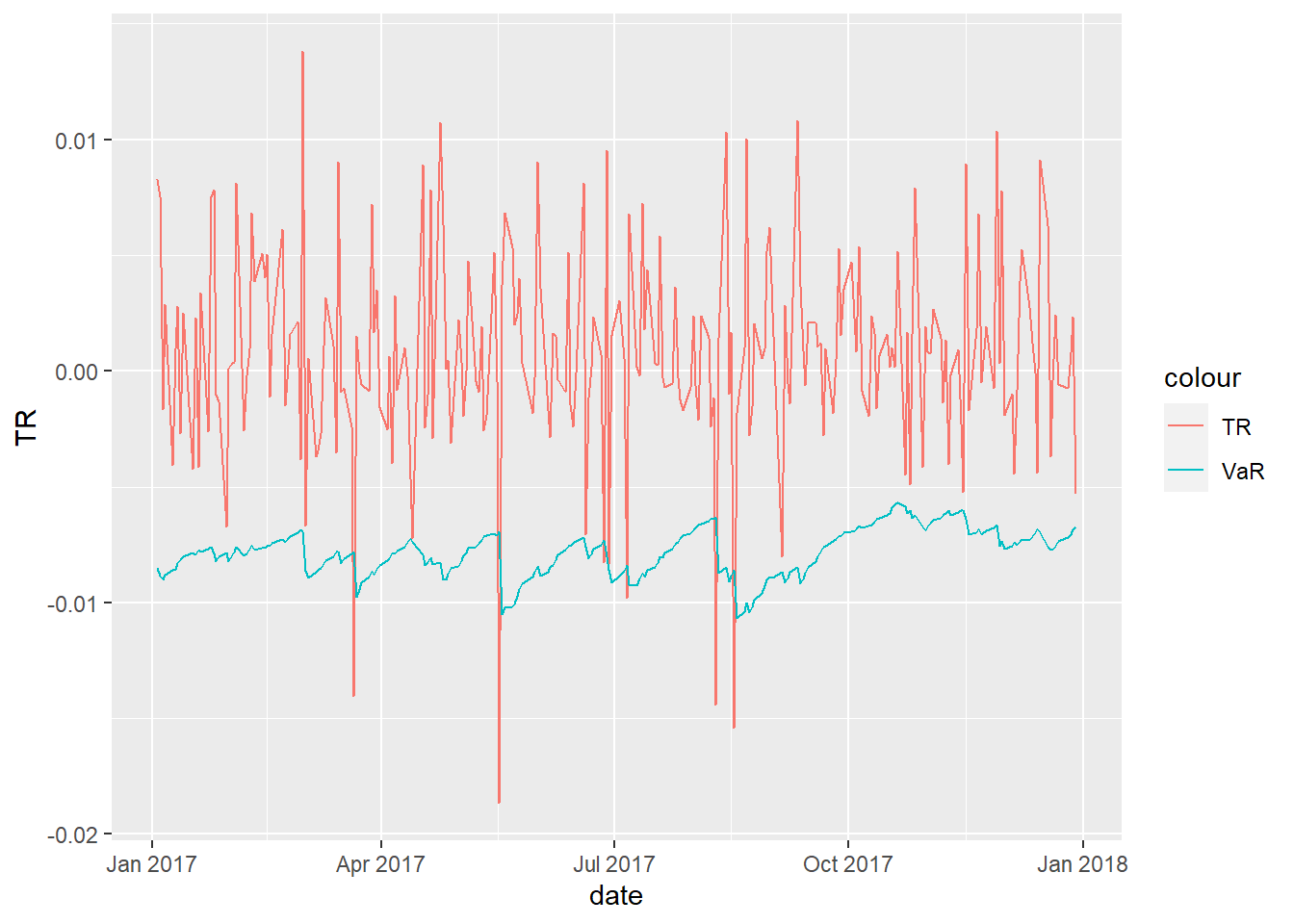
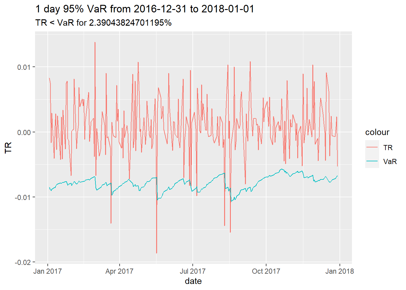
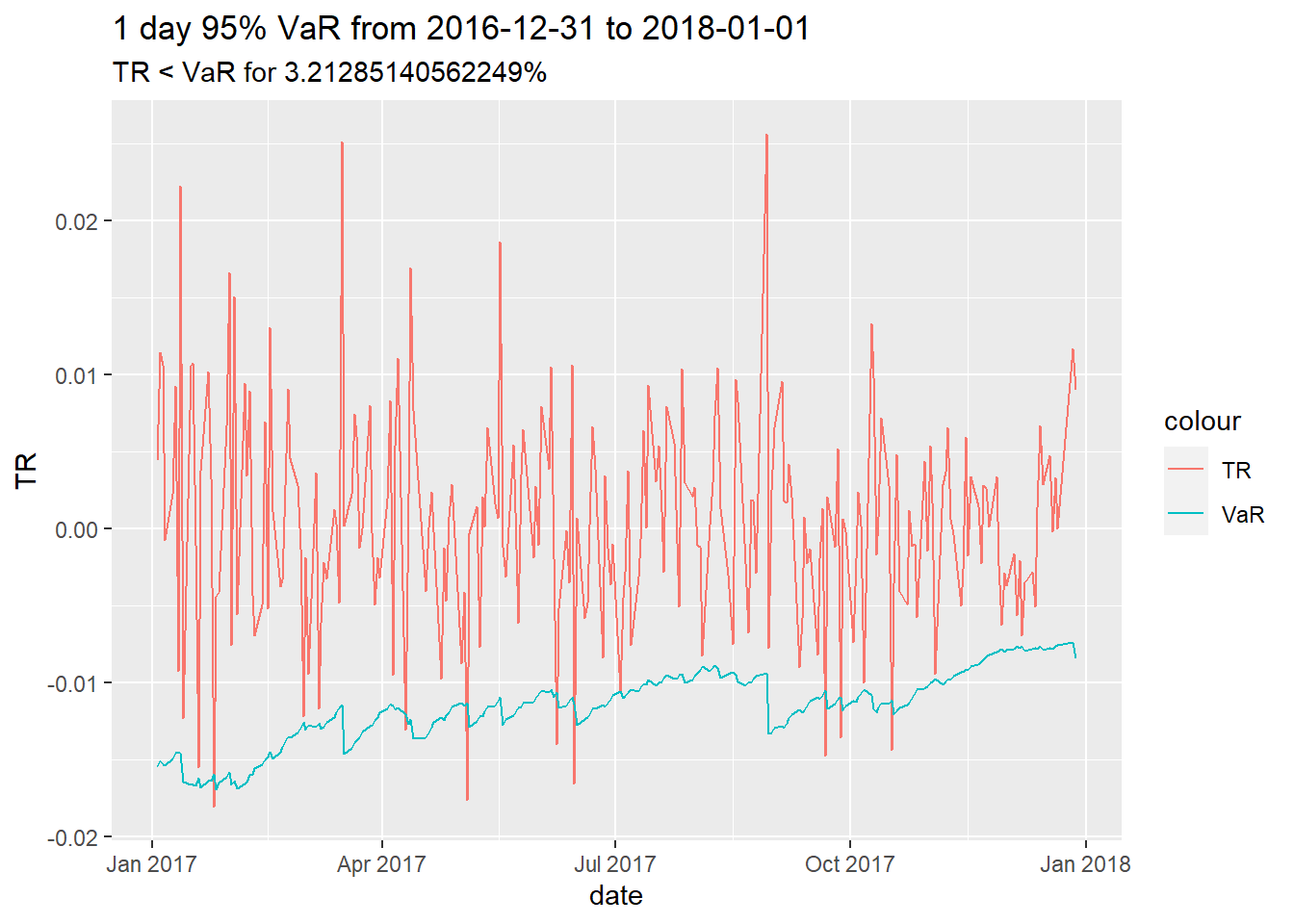
  • VaR and ES from garch take time ordering into account
  • When Fitted values are low => VaR and ES are also low.( Only apply for 1-day)
  • Why is GARCH model better?
    • When volatility is high => Risk is also high => Portfolio manager can take some action to mitigate risk
    • When volatility is low => Risk is low => No action as risk reduction may be costlier to portfolio.
• VaR graph can be produced by using ugarchroll function.
• Summary
  • Basics of Financial risk management
  • Analyze logret of portfolio
  • Distribution: typically non-normal
  • We also have volatility clustering : a behavior typical of asset returns
  • GARCH(1,1)-t can explain both
  • VaR and ES change over time
  • Ideas can be applied to different types of portfolios
    • Margin borrowing: $10 K stocks with
      • $5K your money
      • $5k from a brokerage firm
      • This is a margin position
        • You are hoping to make money from stock price going up
        • Risk -> Price can go down. How much money can you afford to loose -> ES over a time period( like 10 days) with a certain confidence level( like 95%)
    • Stock/Bond Portfolio:
      • Retirement Account
        • 50% US Equities
        • 50% long term corporate bond
        • Plan to retire in 1 year
        • No plan to add more money or take money out next year
        • How much can you loose in 1 year?
        • Can you afford to loose this amount of money for retirement in 1 year?

Imports

library(quantmod)

Loading required package: xts

Loading required package: zoo

Attaching package: 'zoo'

The following objects are masked from 'package:base':

    as.Date, as.Date.numeric

Loading required package: TTR

Registered S3 method overwritten by 'quantmod':
  method            from
  as.zoo.data.frame zoo 

library(ggplot2)
library(purrr) # partial function
library(glue) # string interpolation
library(moments)
library(MASS)
library(metRology)

Attaching package: 'metRology'

The following objects are masked from 'package:base':

    cbind, rbind

library(rugarch)

Loading required package: parallel

Attaching package: 'rugarch'

The following object is masked from 'package:purrr':

    reduce

The following object is masked from 'package:stats':

    sigma

Set Seed.

RNGkind(sample.kind="Rounding") 
set.seed(123789)

Functions

Show the code

filterSeries <- function(s, date_filter="1979-12-31/2017-12-31", new_name='TR'){
  s <- na.omit(s); s
  s <- s[date_filter]; s
  names(s) <- new_name; s
  return(s)
}

getSeries <- function(name, date_filter="1979-12-31/2017-12-31", src='FRED', new_name='TR', auto.assign=FALSE){
  s <- getSymbols(name, src=src, auto.assign = auto.assign); s
  s <- filterSeries(s)
  return(s)
}

get_df <- function(tbl){
  df <- data.frame(date=index(tbl), TR=as.numeric(tbl$TR))
  return(df)
}

logret_1 <- function(tbl){
  return(diff(log(tbl))[-1])
}

aggr_fn <-  function(tbl, fn){
  result <- fn(tbl, sum)
  return(result)
}

logret_w <- partial(aggr_fn, fn = apply.weekly)
logret_m <- partial(aggr_fn, fn = apply.monthly)
logret_q <- partial(aggr_fn, fn = apply.quarterly)
logret_a <- partial(aggr_fn, fn = apply.yearly)

logret_ndays <- function(tbl, days=10){
  len_tbl <-  (nrow(tbl)-days+1)
  new_TR <- sapply(seq(1:len_tbl), function(i){
    sum(tbl[i:(i+days-1)])
    })
  tbl[1:len_tbl]$TR <- new_TR
  return(tbl[1:len_tbl])
}

ret <- function(logret){
  return(exp(logret)-1)
}

get_norm_series <- function(mu, sig, n=100000, set_seed=TRUE){
  if (set_seed){
    RNGkind(sample.kind="Rounding")
    set.seed(123789)
  }

  return(rnorm(n,mu, sig)) 
}

get_sim_series <- function(s, n=100000, set_seed=TRUE){
  if (set_seed){
    RNGkind(sample.kind="Rounding")
    set.seed(123789)
  }

  return(sample(as.vector(s), n, replace=TRUE))
}

get_t_series <- function(mu, sig, df, n=100000, set_seed=TRUE){
  if (set_seed){
    RNGkind(sample.kind="Rounding")
    set.seed(123789)
  }
  return(rt.scaled(n,mean=mu,sd=sig,df=df)) 
}


get_norm_series_from_s <- function(s, n=100000, set_seed=TRUE){
  mu = mean(s)
  sig = sd(s)
  return(get_norm_series(mu, sig, n=n, set_seed = set_seed))
}


get_fit_params  <- function(s){
  fitpars <- s |> as.vector() |> fitdistr(densfun='t') 
  return(fitpars)
}

get_t_series_from_s <- function(s, n=100000, fitpars=NULL, set_seed=TRUE){
  if(is.null(fitpars)){
    fitpars <- s |> get_fit_params()
  }
  t.fit <- fitpars
  return(get_t_series(mu=t.fit$estimate[1], 
                      sig=t.fit$estimate[2], 
                      df=t.fit$estimate[3], 
                      n=n, 
                      set_seed=set_seed))
}

get_sim_VaR <- function(s, alpha=0.05){
  return(quantile(s, alpha) |> unname())
}

get_sim_ES <- function(s, VaR){
  # VaR  <- get_sim_VaR(s, alpha=alpha)
  return(mean(s[s<VaR]))
}

get_VaR <- function(tbl,alpha=0.05){
  mu = mean(tbl)
  sig = sd(tbl)
  VaR = qnorm(alpha, mean=mu, sd=sig) #quantile of normal distribution(only not for any other distribution)
  return(VaR)
}

get_ES <- function(tbl, alpha=0.05){
  mu = mean(tbl)
  sig = sd(tbl)
  ES = mu - sig*dnorm(qnorm(alpha, mean=0, sd=1), 0, 1)/alpha #quantile of normal distribution(only not for any other distribution)
  return(ES)
}

expected_loss <- function(portfolio, risk_num){ #95% confidence that we won't loose more than this amount
  return(portfolio*(exp(risk_num)-1))
}

err <- function(a, b){
  return((a-b)/a*100)
}

get_dist_plot <- function(tbl){
  mu = mean(tbl)
  sig = sd(tbl)
  p <- get_df(tbl) |> 
    ggplot(mapping = aes(x=TR)) +
    geom_histogram(aes(y=after_stat(density)), colour="black", fill="white", 
                 bins=100)+
    geom_density(alpha=.2, fill="violet") +
    geom_vline(aes(xintercept=mu),
            color="brown", linetype="dashed", linewidth=1) + 
    geom_vline(aes(xintercept=mu+2*sig),
            color="brown", linetype="dashed", linewidth=0.1) +
    geom_vline(aes(xintercept=mu-2*sig),
            color="brown", linetype="dashed", linewidth=0.1) +
    labs(title=glue("Distribution of TR: mu={round(mu, 8)}, sigma={round(sig, 8)}"), y='count')
  return(p)
}

get_VaR_plot <- function(tbl, alpha=0.05){
  mu = mean(tbl)
  sig = sd(tbl)
  VaR = qnorm(alpha, mean=mu, sd=sig)
  p <- get_df(tbl) |> 
    ggplot(mapping = aes(x=TR)) +
    geom_histogram(aes(y=after_stat(density)), colour="black", fill="white", 
                 bins=100)+
    geom_density(alpha=.2, fill="violet") +
    geom_vline(aes(xintercept=mu),
            color="brown", linetype="dashed", linewidth=1) + 
    geom_vline(aes(xintercept=VaR),
            color="brown", linewidth=1) +
    labs(title=glue("Distribution of TR: mu: {round(mu, 8)}, sigma: {round(sig, 6)}, VaR({alpha}): {round(VaR, 6)}"), y='count')
  return(p)
}

get_comp_plot <- function(s, alpha=0.05){
  mu <- mean(s)
  sig <- sd(s)
  norm_s <- get_norm_series(mu, sig)
  VaR <- norm_s |> get_sim_VaR(); VaR
  ES <- norm_s |> get_sim_ES(VaR=VaR); ES
  s_sim <- s |> get_sim_series()
  VaR_sim <-  s_sim|>  get_sim_VaR(); VaR_sim
  ES_sim <- s_sim |> get_sim_ES(VaR=VaR_sim); ES_sim
  err_VaR <- err(VaR, VaR_sim) |> round(digits = 2)
  err_ES <- err(ES, ES_sim) |> round(digits = 2)

  
  
  p <- data.frame(TR=s_sim, TR2=norm_s) |> 
    ggplot() +
    geom_density(mapping = aes(x=TR), alpha=.2, fill="violet") +
    geom_density(mapping = aes(x=TR2), alpha=.2, fill="white") +
    geom_vline(aes(xintercept=ES_sim),
            color="brown", linetype="dashed", linewidth=1) + 
    geom_vline(aes(xintercept=ES),
            color="blue", linetype="dashed", linewidth=1) + 
    geom_vline(aes(xintercept=VaR_sim),
            color="brown", linewidth=1) +
    geom_vline(aes(xintercept=VaR),
            color="blue", linewidth=1) +
    labs(title=glue("Distribution of TR alpha({alpha}): \n 
                    VaR_norm(blue): {round(VaR, 6)},VaR_sim(brown): {round(VaR_sim, 6)}, Error: {round(err(VaR, VaR_sim), 2)}% \n 
                    ES_norm: {round(ES, 6)},ES_sim: {round(ES_sim, 6)}, Error: {round(err(ES, ES_sim), 2)}%"), y='count')
  return(p)
}

do_analysis <-  function(s, alpha=0.05){
 
  modelname1 <-  "Norm"
  VaR1 <- s |> get_VaR() |> as.double()
  ES1 <- s |> get_ES() |> as.double()
  # df[nrow(df) + 1,] <- c(modelname, VaR, ES)
  
  modelname2 <-  "NormSim"
  norm_series <- s |> get_norm_series_from_s() 
  VaR2 <- norm_series|> get_sim_VaR(alpha=alpha) |> as.double()
  ES2 <- norm_series |> get_sim_ES(VaR=VaR2) |> as.double()
  # df[nrow(df) + 1,] <- c(modelname, VaR, ES)
  
  modelname3 <-  "T-Sim"
  t_series <- s |> get_t_series_from_s()
  VaR3 <- t_series|> get_sim_VaR(alpha=alpha) |> as.double()
  ES3 <- t_series |> get_sim_ES(VaR=VaR3) |> as.double()
  # df[nrow(df) + 1,] <- c(modelname, VaR, ES)
  
  modelname4 <-  "Sim"
  sim_series <- s |> get_sim_series() 
  VaR4 <- sim_series|> get_sim_VaR(alpha=alpha) |> as.double()
  ES4 <- sim_series |> get_sim_ES(VaR=VaR4) |> as.double()
  
  model_names <- c(modelname1, modelname2, modelname3, modelname4)
  VaRs <- c(VaR1, VaR2, VaR3, VaR4)
  ESs <- c(ES1, ES2, ES3, ES4)

  return(data.frame(ModelName=model_names, VaR=VaRs, ES=ESs))
  
}

get_multi_day_series <- function(s, 
                                 days=10, 
                                 sampling_func=get_sim_series, 
                                 n=100000, 
                                 set_seed=TRUE){
  
  if (set_seed){
    RNGkind(sample.kind="Rounding")
    set.seed(123789)
  }

  rvec <- rep(0, n)
  for( i in 1:days){
    rvec <- rvec + sampling_func(s=s, n=n, set_seed=FALSE)
    # print(rvec |> head())
  }
  return(rvec)
}

get_multi_day_series_block <- function(s,
                                       days=10, 
                                       n=100000, 
                                       set_seed=TRUE){
  
  if (set_seed){
    RNGkind(sample.kind="Rounding")
    set.seed(123789)
  }
  rdat <- s |> as.vector()
  rvec <- rep(0, n)
  posn <- seq(from=1, to=(length(rdat)-days+1), by=1)
  rpos <- sample(posn, size=n, replace=TRUE)
  for( i in 1:days){
    rvec <- rvec + rdat[rpos]
    rpos <- rpos+1 
  }
  return(rvec)
}

do_multi_analysis <-  function(rvec, days=10,  alpha=0.05){
  
  modelname1 <-  glue("student-t({days})")
  fitspars <- rvec |> get_fit_params() #; fitspars
  sampling_func_tdist <-  partial(get_t_series_from_s, 
                                  fitpars = fitspars)
  s1 <-  rvec |> get_multi_day_series(
    sampling_func=sampling_func_tdist)
  VaR1 <- s1 |> get_sim_VaR(alpha=alpha) |> as.double()
  ES1 <- s1 |> get_sim_ES(VaR=VaR1) |> as.double()
  
  modelname2 <-  glue("IID({days})")
  s2 <-  rvec |> get_multi_day_series(days=days)
  VaR2 <- s2 |> get_sim_VaR(alpha=alpha) |> as.double()
  ES2 <- s2 |> get_sim_ES(VaR=VaR2) |> as.double()
  
  modelname3 <-  glue("consecutive({days})")
  s3 <-  rvec |> logret_ndays(days=days) |> get_sim_series(set_seed = TRUE)
  VaR3 <- s3 |> get_sim_VaR(alpha=alpha) |> as.double()
  ES3 <- s3 |> get_sim_ES(VaR=VaR3) |> as.double()
  
  model_names <- c(modelname1, modelname2, modelname3)
  VaRs <- c(VaR1, VaR2, VaR3)
  ESs <- c(ES1, ES2, ES3)

  return(data.frame(ModelName=model_names, VaR=VaRs, ES=ESs))
  
}

expected_loss_df <- function(df, portfolio=1000){
  expected_loss_port = partial(expected_loss, portfolio=portfolio)
  df$VaR <- sapply(df$VaR, expected_loss_port)
  df$ES <- sapply(df$ES, expected_loss_port)
  return(df)
}

Future Vs Historical Distribution

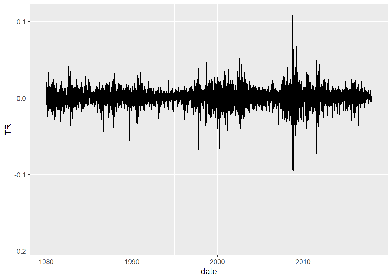
wilsh <- getSeries("WILL5000IND")
wilsh |> head(2)

             TR
1979-12-31 1.90
1980-01-02 1.86

wilsh |> tail(2)

               TR
2017-12-28 124.33
2017-12-29 123.67

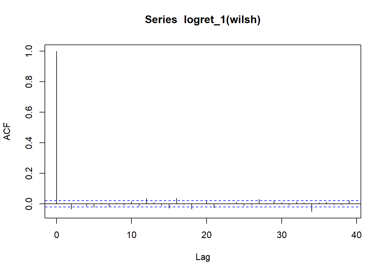
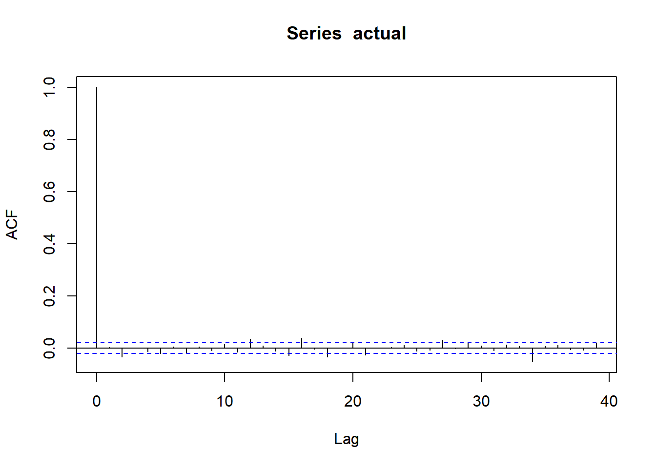
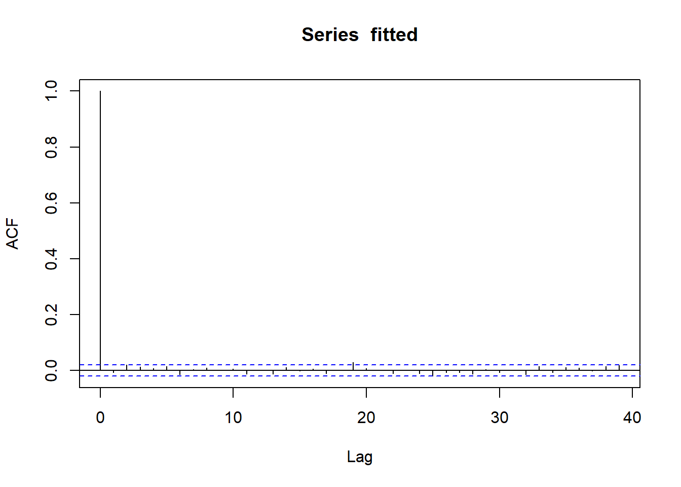
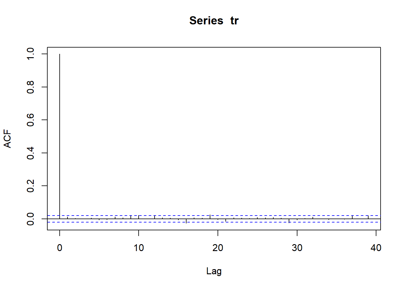
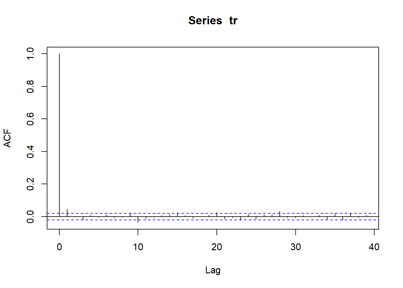
wilsh |> logret_1() |> acf()

ACF Intrepretation

• Dashed lines represent 95% confidence interval for ACF

• If many vertical lines are outside dashed band => We have evidence of serial correlation.

• If all or most lines are inside dashed bands => no strong evidence of serial correlation.

• Above plot shows , We do not find much evidence of serial correlation in the daily log returns of the Wilshire 5000 index. That means the direction of stock prices are not predictable.

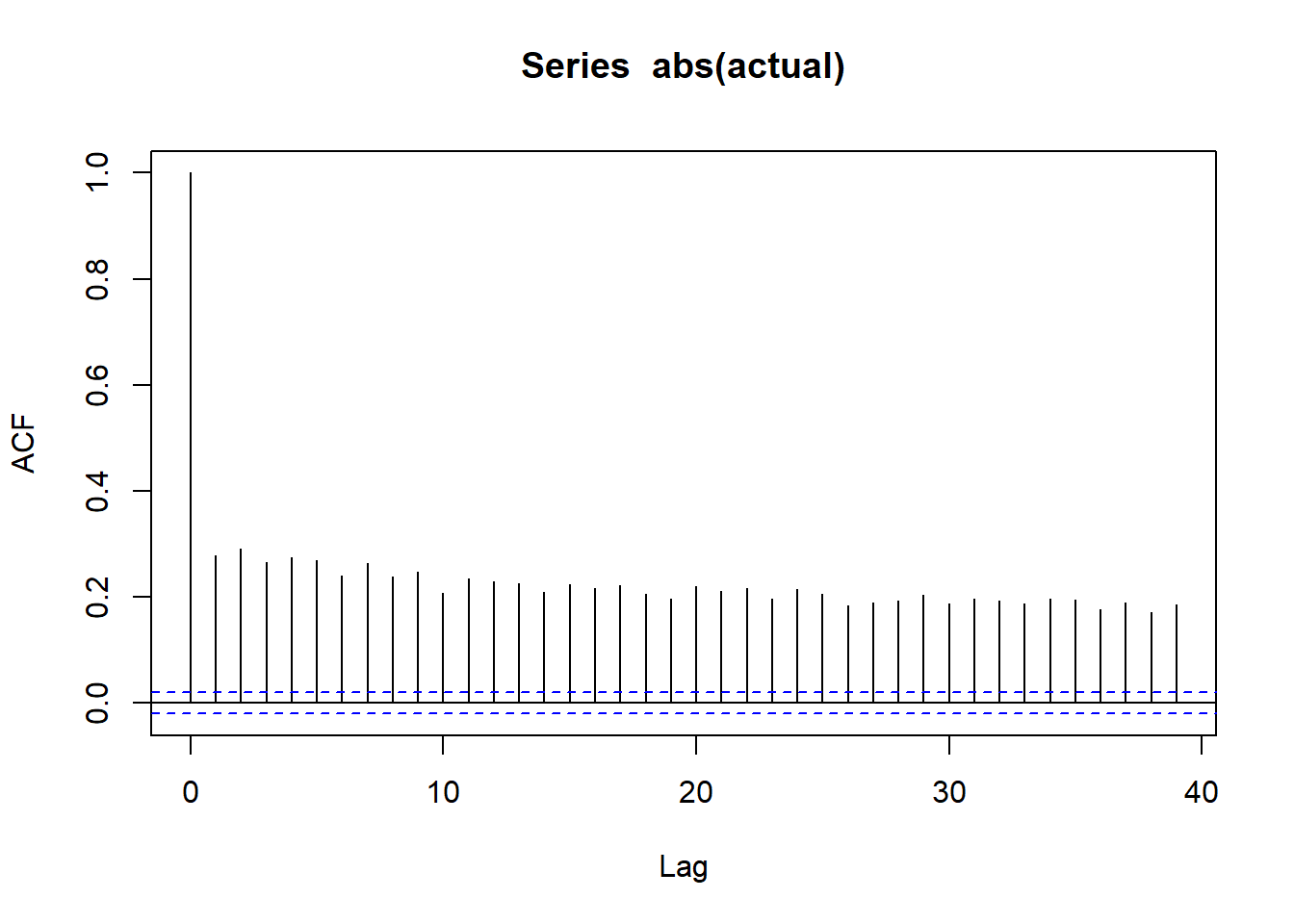
Volatility Clustering

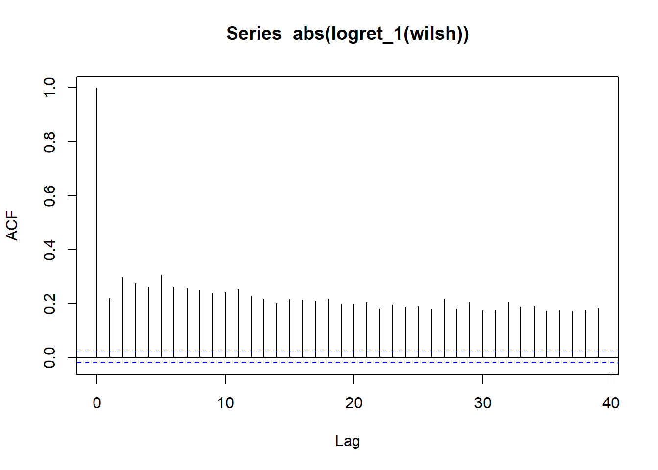
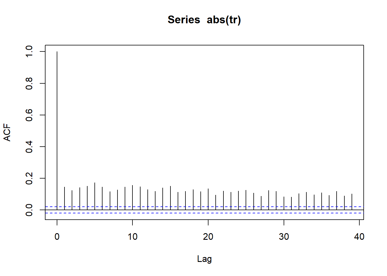
wilsh |> logret_1() |> abs() |> acf()

All lines for autocorrelation on absolute values are above dashed band showing strong possibility of serial correlation and thus volatility clustering

wilsh |> logret_1() |> abs() |> as.vector() |> sample(size=nrow(wilsh)-1) |> acf()

• Shuffled plot shows no serial correlation

• These two plots in combination show strong effect of ordering

Measuring effect/importance of ordering for volatility clustering

tr <- wilsh |> logret_1()
shuffled_tr <- tr
shuffled_s <- tr |> as.vector() |> sample(size=nrow(tr))
shuffled_tr$TR <- shuffled_s

tr |>
  get_df() |>
  ggplot(mapping = aes(x = date, y=TR)) +
  geom_line()
shuffled_tr |>
  get_df() |>
  ggplot(mapping = aes(x = date, y=TR)) +
  geom_line()
tr |> abs() |> acf()
shuffled_tr |> abs() |> acf()

Actual TR

Permutation TR

Actual TR ACF

Permutation TR ACF

GARCH model

GARCH (1,1) - normal model

How to use rugarch package?

• Specify the GARCH model using the ‘ugrachspec’ function

• Then specify

  • variance.model

  • mean.model

  • distribution.model

logret <- wilsh |> logret_1()
garch.N <- ugarchspec(variance.model=list(model='sGARCH', garchOrder=c(1,1)),
                      mean.model = list(armaOrder = c(0,0), include.mean=TRUE),
                      distribution.model = "norm"); garch.N

*---------------------------------*
*       GARCH Model Spec          *
*---------------------------------*

Conditional Variance Dynamics   
------------------------------------
GARCH Model     : sGARCH(1,1)
Variance Targeting  : FALSE 

Conditional Mean Dynamics
------------------------------------
Mean Model      : ARFIMA(0,0,0)
Include Mean        : TRUE 
GARCH-in-Mean       : FALSE 

Conditional Distribution
------------------------------------
Distribution    :  norm 
Includes Skew   :  FALSE 
Includes Shape  :  FALSE 
Includes Lambda :  FALSE 

fit.garch.N <- ugarchfit(spec = garch.N, data=logret); fit.garch.N

*---------------------------------*
*          GARCH Model Fit        *
*---------------------------------*

Conditional Variance Dynamics   
-----------------------------------
GARCH Model : sGARCH(1,1)
Mean Model  : ARFIMA(0,0,0)
Distribution    : norm 

Optimal Parameters
------------------------------------
        Estimate  Std. Error  t value Pr(>|t|)
mu      0.000678    0.000079   8.5856 0.000000
omega   0.000002    0.000001   2.8917 0.003832
alpha1  0.090834    0.007943  11.4364 0.000000
beta1   0.893290    0.008580 104.1170 0.000000

Robust Standard Errors:
        Estimate  Std. Error  t value Pr(>|t|)
mu      0.000678    0.000086  7.89699  0.00000
omega   0.000002    0.000006  0.30107  0.76336
alpha1  0.090834    0.060970  1.48981  0.13627
beta1   0.893290    0.071761 12.44813  0.00000

LogLikelihood : 31772.43 

Information Criteria
------------------------------------
                    
Akaike       -6.6302
Bayes        -6.6272
Shibata      -6.6302
Hannan-Quinn -6.6291

Weighted Ljung-Box Test on Standardized Residuals
------------------------------------
                        statistic   p-value
Lag[1]                      24.81 6.342e-07
Lag[2*(p+q)+(p+q)-1][2]     24.81 2.438e-07
Lag[4*(p+q)+(p+q)-1][5]     27.70 1.402e-07
d.o.f=0
H0 : No serial correlation

Weighted Ljung-Box Test on Standardized Squared Residuals
------------------------------------
                        statistic p-value
Lag[1]                     0.3101  0.5776
Lag[2*(p+q)+(p+q)-1][5]    2.8686  0.4316
Lag[4*(p+q)+(p+q)-1][9]    3.7794  0.6264
d.o.f=2

Weighted ARCH LM Tests
------------------------------------
            Statistic Shape Scale P-Value
ARCH Lag[3]   0.01043 0.500 2.000  0.9186
ARCH Lag[5]   0.01799 1.440 1.667  0.9989
ARCH Lag[7]   0.75403 2.315 1.543  0.9500

Nyblom stability test
------------------------------------
Joint Statistic:  179.7119
Individual Statistics:               
mu      0.06819
omega  22.32490
alpha1  0.13086
beta1   0.19771

Asymptotic Critical Values (10% 5% 1%)
Joint Statistic:         1.07 1.24 1.6
Individual Statistic:    0.35 0.47 0.75

Sign Bias Test
------------------------------------
                   t-value      prob sig
Sign Bias            2.182 2.915e-02  **
Negative Sign Bias   2.016 4.384e-02  **
Positive Sign Bias   2.799 5.130e-03 ***
Joint Effect        48.248 1.886e-10 ***


Adjusted Pearson Goodness-of-Fit Test:
------------------------------------
  group statistic p-value(g-1)
1    20     478.2    2.065e-89
2    30     418.6    1.241e-70
3    40     813.1   1.962e-145
4    50     782.4   8.811e-133


Elapsed time : 0.4649279 

save1 <- cbind(logret, fit.garch.N@fit$sigma, fit.garch.N@fit$z)
names(save1) <- c('logret','s','z')
save1

                  logret           s           z
1980-01-02 -0.0212773984 0.010722744 -2.04757252
1980-01-04  0.0106952891 0.012172801  0.82290777
1980-01-07  0.0053050522 0.011965039  0.38669792
1980-01-08  0.0209431738 0.011467887  1.76710648
1980-01-09  0.0000000000 0.012508564 -0.05421857
1980-01-10  0.0103093697 0.011895049  0.80967916
1980-01-11  0.0000000000 0.011683400 -0.05804787
1980-01-14  0.0051151007 0.011120254  0.39899305
1980-01-15  0.0050890695 0.010674035  0.41323391
1980-01-16  0.0000000000 0.010258012 -0.06611383
       ...                                      
2017-12-15  0.0091079755 0.005269317  1.59978602
2017-12-18  0.0062944043 0.005739355  0.97854343
2017-12-19 -0.0037072899 0.005828619 -0.75240576
2017-12-20 -0.0004037957 0.005811807 -0.18617137
2017-12-21  0.0024203320 0.005653465  0.30815359
2017-12-22 -0.0005642204 0.005523522 -0.22493200
2017-12-26 -0.0007258943 0.005392257 -0.26039017
2017-12-27  0.0008065167 0.005275921  0.02432186
2017-12-28  0.0023352267 0.005152582  0.32159219
2017-12-29 -0.0053225932 0.005064389 -1.18489903

glue("{fit.garch.N@model$modeldesc$vmodel}-{fit.garch.N@model$modeldesc$distno}-{fit.garch.N@model$modeldesc$distribution}")

sGARCH-1-norm

g <- save1$z
g |> as.vector() |> mean() |> round(digits=4)

[1] -0.0309

g |> as.vector() |> sd() |> round(digits=4)

[1] 1.0006

g |> as.vector() |> skewness() |> round(digits=2)

[1] -0.59

g |> as.vector() |> kurtosis() |> round(digits=2)

[1] 6.44

g |> as.vector() |> jarque.test()

    Jarque-Bera Normality Test

data:  as.vector(g)
JB = 5292.3, p-value < 2.2e-16
alternative hypothesis: greater

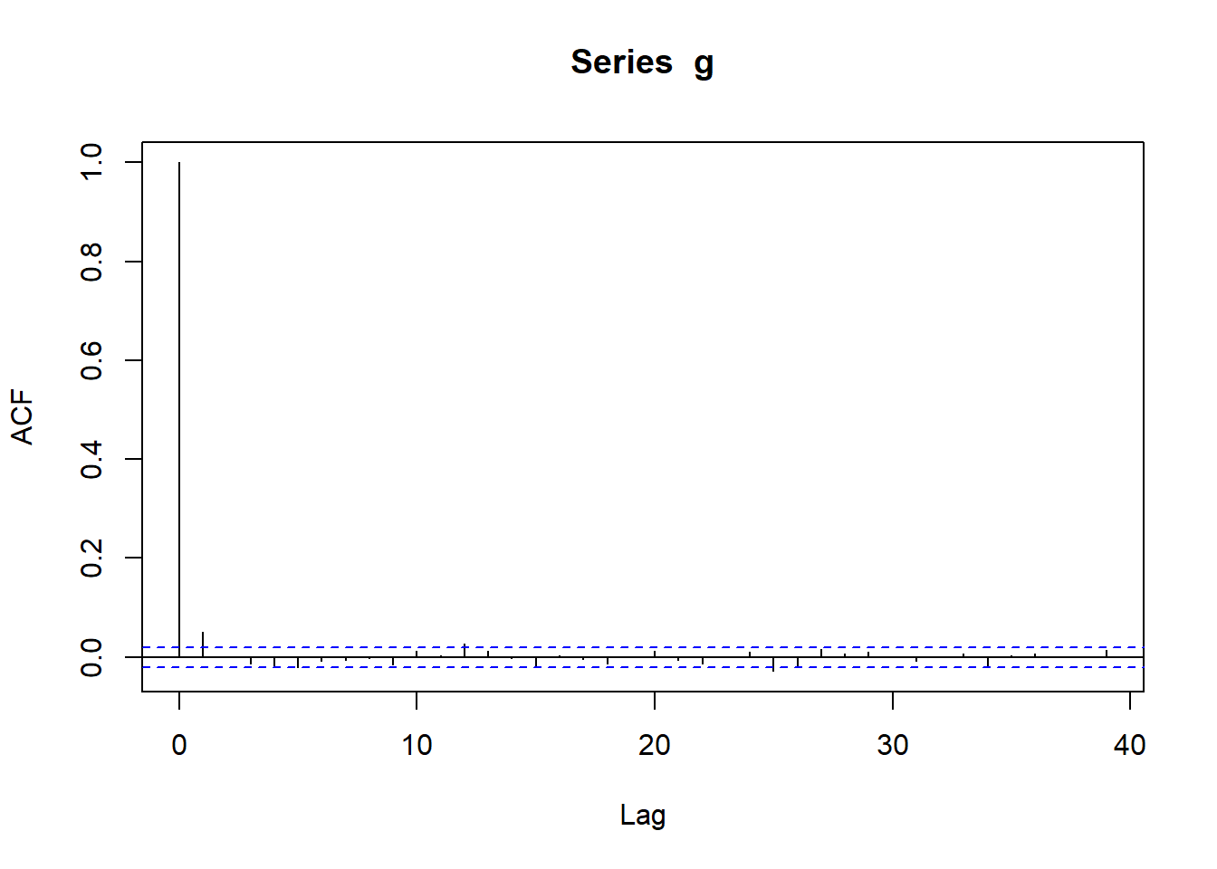
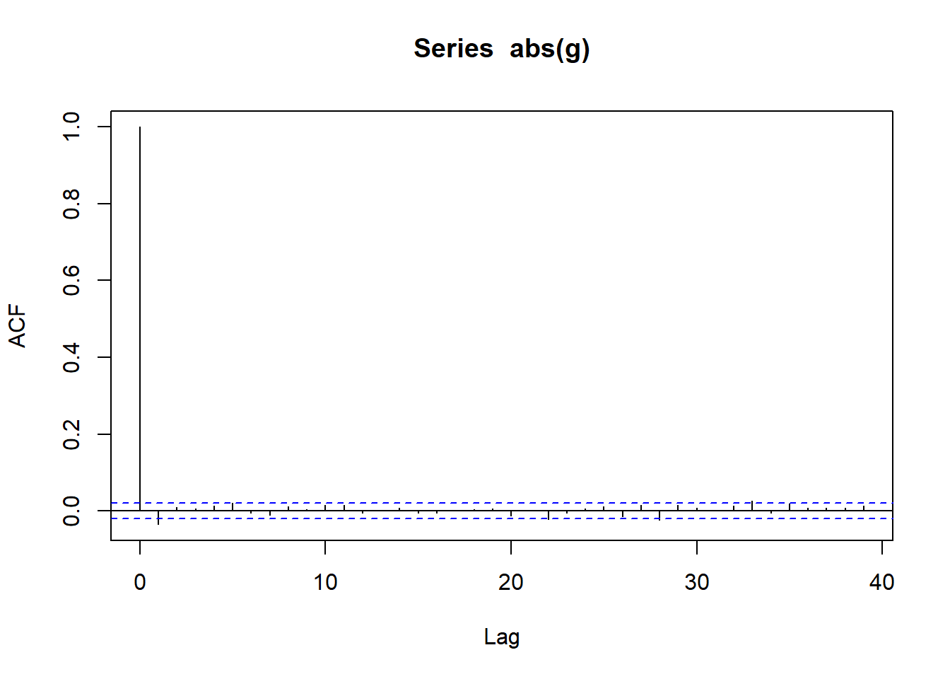
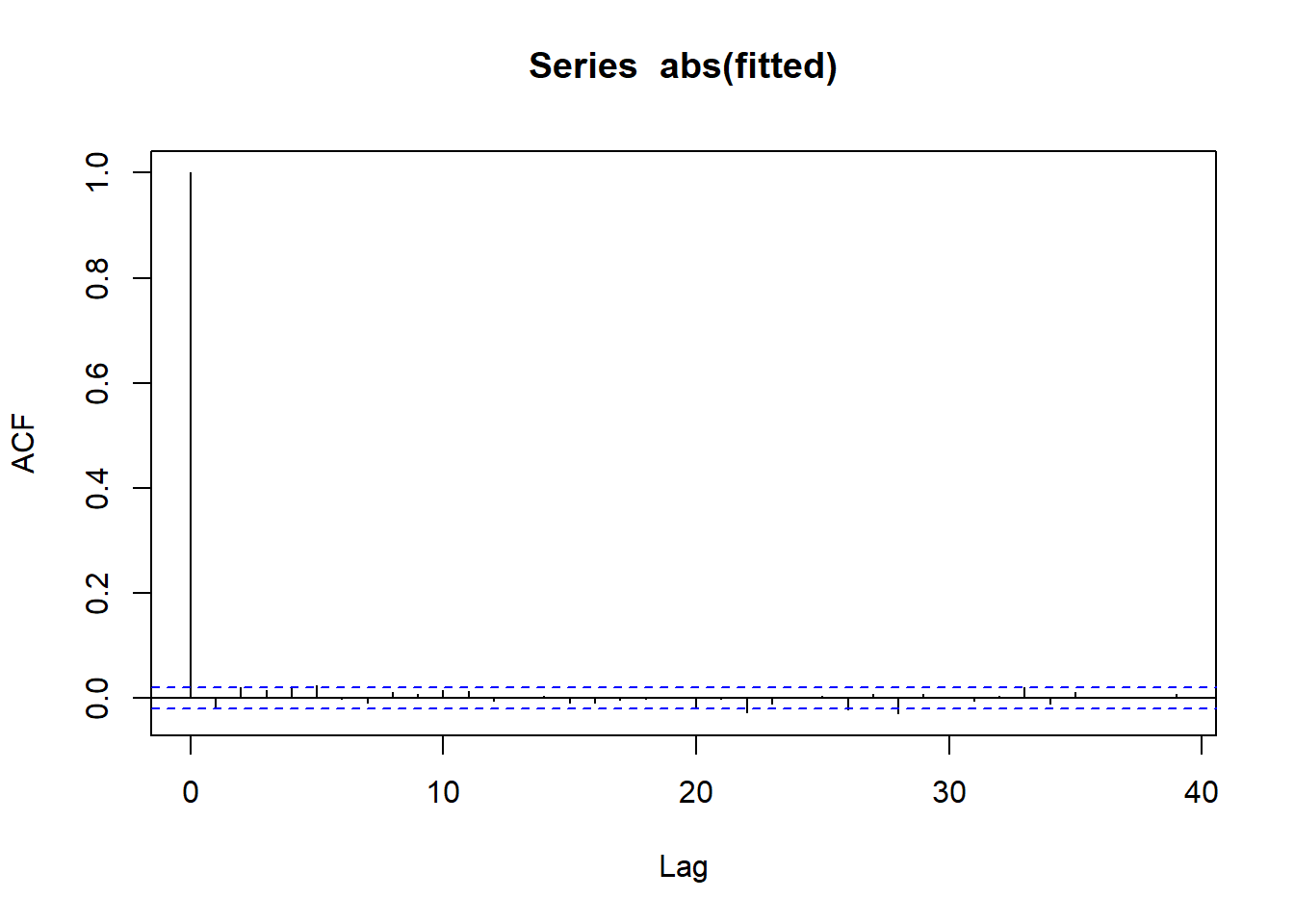
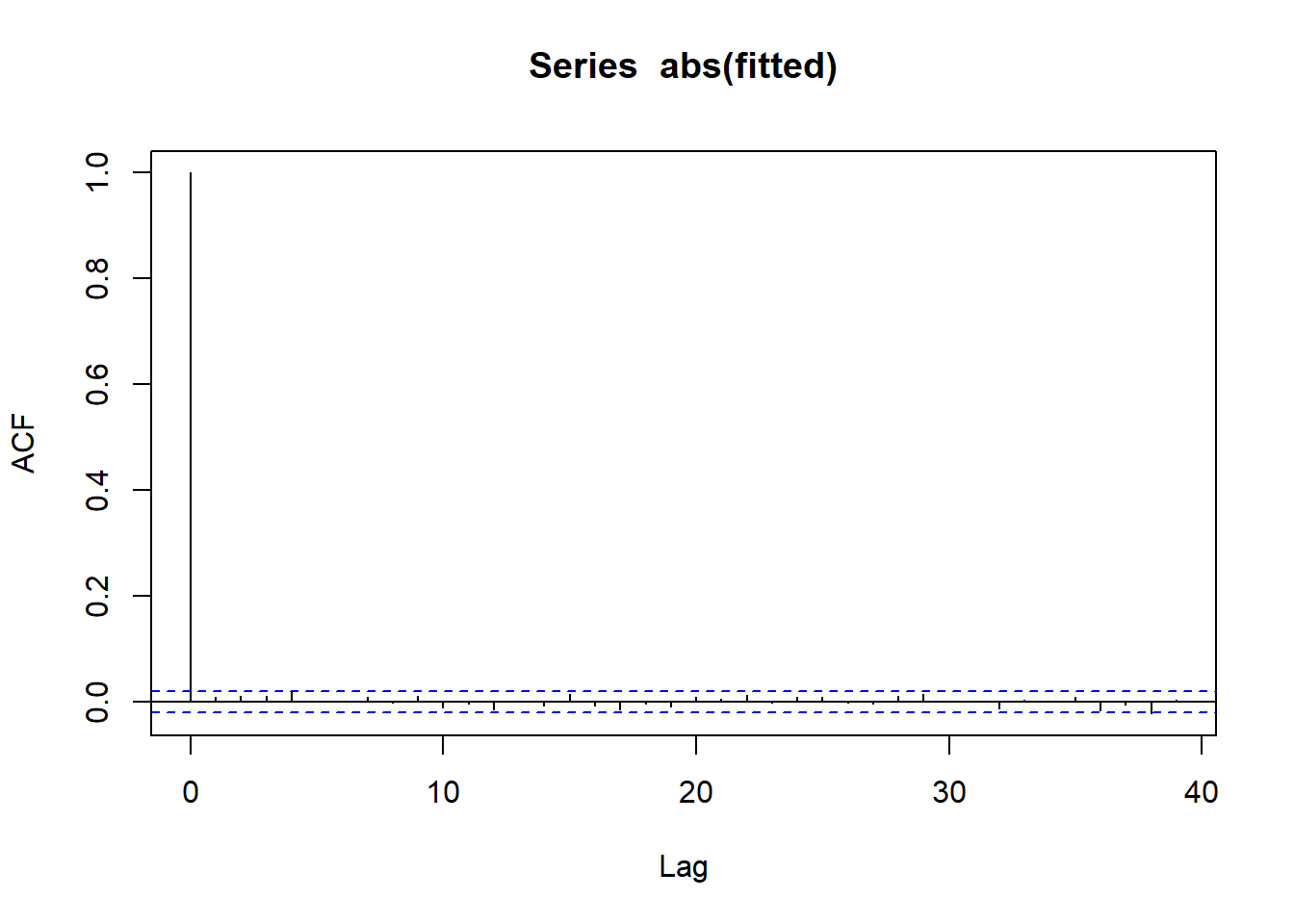
g |> acf()
g |> abs() |> acf()

ACF of fitted e(t)

ACF of |fitted e(t)|

g <- save1$logret
g |> as.vector() |> mean() |> round(digits=4)

[1] 4e-04

g |> as.vector() |> sd() |> round(digits=4)

[1] 0.0107

g |> as.vector() |> skewness() |> round(digits=2)

[1] -0.91

g |> as.vector() |> kurtosis() |> round(digits=2)

[1] 21.8

g |> as.vector() |> jarque.test()

    Jarque-Bera Normality Test

data:  as.vector(g)
JB = 142514, p-value < 2.2e-16
alternative hypothesis: greater

t <- g |> as.vector() |> jarque.test()
t$statistic

      JB 
142514.5 

t$p.value

[1] 0

t$alternative

[1] "greater"

Interpretation of Garch(1,1) - normal model

• For a normal distribution to be true fitted e(t) should have

  • mean=0, sd=1, skewness=0, kurtosis=3

  • Jacque bera test should be able to confirm normality

• Kurtosis of our data is around 21.8 . Our fitted distribution is around 6.44 and normal distribution expects it to be 3 => GARCH model is able to explain quite a lot but not all of the heavy tail

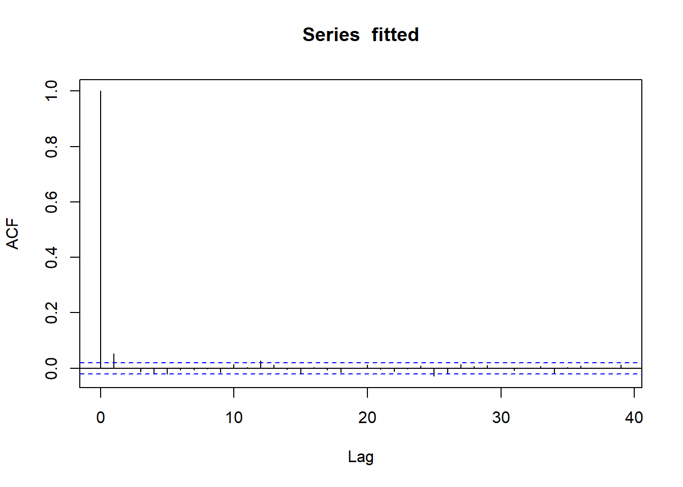
• ACF curves for fitted value indicated no serial correlation

• ACF curves for absolute fitted value indicate no serial correlation and thus, no volatility clustering => Variance equation in GARCH model is able to explain all volatility clustering in our data

• Conclusion: GARCH(1,1) - normal model can explain

  • Volatility clustering of our data

  • Some but not all of heavy tails of the data

  • To have better explanation of distribution we need to change distribution equation.

get_fit_params_garch  <- function(s, spec=NULL, solver="solnp"){
  if(is.null(spec)){
    spec <- ugarchspec(variance.model=list(model='sGARCH', garchOrder=c(1,1)),
                      mean.model = list(armaOrder = c(0,0), include.mean=TRUE),
                      distribution.model = "std")
  }
  fit.garch.dist <- ugarchfit(spec = spec, data=s, solver=solver)
  return(fit.garch.dist)
}

s <- wilsh |> logret_1(); s |> head()

                     TR
1980-01-02 -0.021277398
1980-01-04  0.010695289
1980-01-07  0.005305052
1980-01-08  0.020943174
1980-01-09  0.000000000
1980-01-10  0.010309370

fit.garch <- s |> get_fit_params_garch(); s |> head()

                     TR
1980-01-02 -0.021277398
1980-01-04  0.010695289
1980-01-07  0.005305052
1980-01-08  0.020943174
1980-01-09  0.000000000
1980-01-10  0.010309370

Explainability_dist_model

explainability_dist_model <- function(s, spec=NULL, solver="solnp"){
  fit.garch <- s |> get_fit_params_garch(spec=spec, solver=solver)
  save <- cbind(s, fit.garch@fit$sigma, fit.garch@fit$z)
  names(save) <- c('logret','s', 'z')
  models <- c("Norm", "Actual",
              glue("{fit.garch@model$modeldesc$vmodel}-{fit.garch@model$modeldesc$distno}-{fit.garch@model$modeldesc$distribution}"))
  
  means <- c(0, save$logret |> mean(), save$z |> mean())
  sds <- c(1, save$logret |> sd(), save$z |> sd())
  skewnesss  <- c(0, save$logret |> skewness(), save$z |> skewness()) 
  kurtosiss <- c(3, save$logret |> kurtosis(), save$z |> kurtosis()) 
  jb_actual  <- save$logret |> as.vector() |> jarque.test()
  jb_dist <- save$z |> as.vector() |> jarque.test()
  JBSTAT.stat <- c("", jb_actual$statistic, jb_dist$statistic )
  JBSTAT.pvalue <- c("", jb_actual$p.value, jb_dist$p.value )
  JBSTAT.alternative <- c("", jb_actual$alternative, jb_dist$alternative)
  df <- data.frame( mean = means,
                    sd = sds,
                    skewness = skewnesss,
                    kurtosis = kurtosiss,
                    JBSTAT.stat = JBSTAT.stat,
                    JBSTAT.pvalue = JBSTAT.pvalue,
                    JBSTAT.alternative = JBSTAT.alternative)
  row.names(df) <- models
  
  out <- list(save = save, df=df, parm=fit.garch@fit$coef)
  return(out)
}

out <- wilsh |> logret_1() |> explainability_dist_model()

out$parm

          mu        omega       alpha1        beta1        shape 
7.906871e-04 7.955355e-07 7.125105e-02 9.228052e-01 6.140006e+00 

out$df |> format(digits=4)

fitted <-  out$save$z
fitted |> acf()
fitted |> abs() |> acf()
actual<-  out$save$logret
actual |> acf()
actual |> abs() |> acf()

ACF of fitted e(t)

ACF of |fitted e(t)|

ACF of actual e(t)-Series Correlation

ACF of |actual e(t)|-Volatility Clustering

df <- data.frame(date=index(out$save), 
           s=as.numeric(out$save$s), 
           TR=as.numeric(out$save$logret)) 
ggplot(data=df) + geom_line(mapping = aes(x=date, y=s))
ggplot(data=df) + geom_line(mapping = aes(x=date, y=TR))

STD

Returns

Exercise 12

load("W1_Exercise2_FRED_gold.gz")

g <- gold |> filterSeries() |> logret_1()
g |> head(2)

                    TR
1980-01-03  0.12500543
1980-01-04 -0.07532201

g |> tail(2)

                    TR
2017-12-27 0.011674890
2017-12-28 0.009025894

out <- g |> explainability_dist_model() 
out$parm |> round(digits=6)

      mu    omega   alpha1    beta1    shape 
0.000020 0.000000 0.058965 0.940035 4.705043 

out$df |> format(digits=4)

fitted <-  out$save$z
fitted |> acf()
fitted |> abs() |> acf()
actual<-  out$save$logret
actual |> acf()
actual |> abs() |> acf()

ACF of fitted e(t)

ACF of |fitted e(t)|

ACF of actual e(t)-Series Correlation

ACF of |actual e(t)|-Volatility Clustering

VaR and ES for GARCH Bootstrap

get_garch_series_from_s <- function(s, n=100000, fitpars=NULL, set_seed=TRUE, solver="solnp"){
  
  if (set_seed){
    RNGkind(sample.kind="Rounding")
    set.seed(123789)
  }
  if(is.null(fitpars)){
    fitpars <- s |> get_fit_params_garch(solver = solver)
  }
  
  boot.garch  <- ugarchboot(fitpars, 
                            method = "Partial",
                            sampling="raw",
                            n.ahead=1,
                            n.bootpred = n,
                            solver="solnp"
                            )
  return(boot.garch@fseries |> as.vector())
}

VaR and ES nextday (Jan2, 2018) with 95% CI

logret <- wilsh |> logret_1() 
s  <- logret |> get_garch_series_from_s()

wilsh |> head(1) |> index()

[1] "1979-12-31"

wilsh |> tail(1) |> index()

[1] "2017-12-29"

VaR <-  s |> get_sim_VaR(alpha=0.05); VaR

[1] -0.007456152

ES <- s |> get_sim_ES(VaR=VaR);ES

[1] -0.01094603

VaR and ES nextday (Oct19, 1987) with 95% CI

logret <- wilsh |> logret_1() |> filterSeries(date_filter = '1979-12-31/1987-10-19')
s  <- logret |> get_garch_series_from_s()

logret |> head(1) |> index()

[1] "1980-01-02"

logret |> tail(1) |> index()

[1] "1987-10-19"

VaR <-  s |> get_sim_VaR(alpha=0.05); VaR

[1] -0.07382125

ES <- s |> get_sim_ES(VaR=VaR);ES

[1] -0.1058245

GARCH 1day many input model

• 2008-09-15 -Lehmann failure

• 1987-10-19 - Largest single day decline in US stock market

do_analysis_garch_nextday <- function(rvec, 
                                      date.start="1979-12-31",
                                      date.ends=c("2017-12-29"),
                                      fitspar=NULL,
                                      n=100000,
                                      alpha=0.05,
                                      solver="solnp"){
  
  VaRs <- list()
  ESs <- list()
  for(i in date.ends){
    filter_str = glue('{date.start}/{i}')
    rvec_filter <- rvec |> filterSeries(date_filter=filter_str)
    s <- rvec_filter |> get_garch_series_from_s(fitpars=fitspar, 
                                                n=n, 
                                                solver=solver)
    VaR <-  s |> get_sim_VaR(alpha=alpha)
    ES <- s |> get_sim_ES(VaR=VaR)
    VaRs <- c(VaRs, VaR)
    ESs <- c(ESs,ES)
  }
  
  return(data.frame(day=date.ends |> as.Date(),
                    Var=VaRs |> as.double(),
                    ES=ESs |> as.double()))
}

wilsh |> logret_1() |> do_analysis_garch_nextday(date.ends=c("2017-12-29","2008-09-15","1987-10-19")) |> format(digits=4)

Rolling 1-day VaR

s <- wilsh |> logret_1()
spec <- ugarchspec(variance.model=list(model='sGARCH', garchOrder=c(1,1)),
                   mean.model = list(armaOrder = c(0,0), include.mean=TRUE),
                   distribution.model = "std")

s2016 <- s |> filterSeries(date_filter = '1980-01-01/2016-12-31')
n2016 <- length(s2016); n2016

[1] 9332

roll.garch <- ugarchroll(spec=spec,
                         data=s,
                         start=1,
                         n.ahead=1,
                         n.start =n2016,
                         forecast.length=1,
                         refit.every = 100,
                         refit.window = "recursive",
                         calculate.VaR = TRUE,
                         VaR.alpha = 0.05,
                         keep.coef = TRUE)

roll.garch@forecast$VaR |> head(1)

roll.garch@forecast$VaR |> tail(1)

s_from2017 <- s |> filterSeries(date_filter = '2016-12-31/2018-01-01')
s_from2017 |> head(1)

                    TR
2017-01-03 0.008281823

s_from2017 |> tail(1)

                     TR
2017-12-29 -0.005322593

roll_df <- data.frame(date=index(s_from2017), TR=s_from2017$TR, VaR=roll.garch@forecast$VaR[1])

colnames(roll_df) <- c('date', 'TR', 'VaR')
roll_df

sum(roll_df$TR < roll_df$VaR)*100/nrow(roll_df) |> round(digits=1)

[1] 2.390438

roll.garch@forecast$VaR[1] |> head(5) |> as.vector() 

$`alpha(5%)`
[1] -0.008529988 -0.008837648 -0.009013061 -0.008797251 -0.008579853

ggplot(data=roll_df)+ 
  geom_line(mapping = aes(x=date, y=TR, color='TR')) +
  geom_line(mapping = aes(x=date, y=VaR, color='VaR'))

get_garch_VaR_plot <- function(s, 
                               spec=NULL, 
                               alpha=0.05,
                               refit.every=1,
                               date.start='1979-12-31', 
                               date.fit='2016-12-31', 
                               date.predict='2018-01-01'){
  if(is.null(spec)){
    spec = ugarchspec(variance.model=list(model='sGARCH', garchOrder=c(1,1)),
                   mean.model = list(armaOrder = c(0,0), include.mean=TRUE),
                   distribution.model = "std")
  }
  
  sfit <- s |> filterSeries(date_filter = glue('{date.start}/{date.fit}'))
  nfit <- length(sfit)
  roll.garch <- ugarchroll(spec=spec,
                         data=s,
                         start=1,
                         n.ahead=1,
                         n.start=nfit,
                         forecast.length=1,
                         refit.every = refit.every,
                         refit.window = "recursive",
                         calculate.VaR = TRUE,
                         VaR.alpha = alpha,
                         keep.coef = TRUE)
  
  spredict <- s |> filterSeries(date_filter = glue('{date.fit}/{date.predict}'))
  roll_df <- data.frame(date=index(spredict), 
                        TR=spredict$TR, 
                        VaR=roll.garch@forecast$VaR[1])
  colnames(roll_df) <- c('date', 'TR', 'VaR')
  
  p <- ggplot(data=roll_df)+ 
    geom_line(mapping = aes(x=date, y=TR, color='TR')) +
    geom_line(mapping = aes(x=date, y=VaR, color='VaR')) +
    labs(title=glue("1 day {(1-alpha)*100}% VaR from {date.fit} to {date.predict}" ), subtitle = glue("TR < VaR for {sum(roll_df$TR < roll_df$VaR)*100/nrow(roll_df)}%") )
  return(p)
  
}

wilsh |> logret_1() |> get_garch_VaR_plot(refit.every = 100, alpha = 0.05)

Exercise 13

g <- gold |> filterSeries() |> logret_1()
g |> head(2)

                    TR
1980-01-03  0.12500543
1980-01-04 -0.07532201

g |> tail(2)

                    TR
2017-12-27 0.011674890
2017-12-28 0.009025894

g |> do_analysis_garch_nextday(date.ends=c("2017-12-29","2008-09-15","1987-10-19")) |> format(digits=5)

Warning in RNGkind(sample.kind = "Rounding"): non-uniform 'Rounding' sampler
used

Warning in RNGkind(sample.kind = "Rounding"): non-uniform 'Rounding' sampler
used

Warning in RNGkind(sample.kind = "Rounding"): non-uniform 'Rounding' sampler
used

g |> get_garch_VaR_plot(refit.every = 100, alpha = 0.05)

Quiz 1

us2yen <-getSeries("DEXJPUS")
yen2us <- 1/us2yen 
yen2us |> head(2)

                    TR
1979-12-31 0.004161465
1980-01-02 0.004193751

yen2us |> tail(2)

                    TR
2017-12-28 0.008861320
2017-12-29 0.008873902

tr <- yen2us |> logret_1()
tr |> acf()

tr <- yen2us |> logret_1()
shuffled_tr <- tr
shuffled_s <- tr |> as.vector() |> sample(size=nrow(tr))
shuffled_tr$TR <- shuffled_s

tr |>
  get_df() |>
  ggplot(mapping = aes(x = date, y=TR)) +
  geom_line()

shuffled_tr |>
  get_df() |>
  ggplot(mapping = aes(x = date, y=TR)) +
  geom_line()

tr |> abs() |> acf()

shuffled_tr |> abs() |> acf()

s <- yen2us |> logret_1() 

spec <- ugarchspec(variance.model=list(model='sGARCH', garchOrder=c(1,1)),
                  mean.model = list(armaOrder = c(0,0), include.mean=TRUE),
                  distribution.model = "std")
fit.garch <- ugarchfit(spec = spec, data=s, solver = 'hybrid',
                            solver.control = list(),
                            fit.control = list(stationarity = 1, 
                                               fixed.se = 0,
                                               scale = 0, 
                                               rec.init = 'all',
                                               trunclag = 1000) )
save <- cbind(s, fit.garch@fit$sigma, fit.garch@fit$z)
names(save) <- c('logret','s', 'z')
fit.garch@fit$coef

           mu         omega        alpha1         beta1         shape 
-9.894718e-05  1.079617e-07  3.294518e-02  9.661616e-01  4.960222e+00 

out <- yen2us |> logret_1() |> explainability_dist_model(solver="hybrid")
out$parm |> round(digits=6)

       mu     omega    alpha1     beta1     shape 
-0.000099  0.000000  0.032945  0.966162  4.960222 

yen2us |> logret_1() |> do_analysis_garch_nextday(date.ends=c("2018-01-01","2008-09-15","1987-10-19"), solver='hybrid') |> format(digits=4)

Warning in RNGkind(sample.kind = "Rounding"): non-uniform 'Rounding' sampler
used

Warning in RNGkind(sample.kind = "Rounding"): non-uniform 'Rounding' sampler
used

Warning in RNGkind(sample.kind = "Rounding"): non-uniform 'Rounding' sampler
used

yen2us |> logret_1() |> tail(1)

                    TR
2017-12-29 0.001418817

yen2us |> logret_1() |> do_analysis_garch_nextday(date.ends=c("2017-12-29"), solver='hybrid') |> format(digits=4)

Warning in RNGkind(sample.kind = "Rounding"): non-uniform 'Rounding' sampler
used

Quiz 2

bp2us <-getSeries("DEXUSUK")
bp2us |> head(2)

               TR
1979-12-31 2.2185
1980-01-02 2.2427

bp2us |> tail(2)

               TR
2017-12-28 1.3450
2017-12-29 1.3529

# yen2us <- 1/us2yen 
# yen2us |> head(2)
# yen2us |> tail(2)

s <- bp2us |> logret_1()
s |> head(2)

                     TR
1980-01-02  0.010849205
1980-01-03 -0.001204631

s |> tail(2)

                    TR
2017-12-28 0.003500544
2017-12-29 0.005856424

tr <- bp2us |> logret_1()
tr |> acf()

tr <- bp2us |> logret_1()
shuffled_tr <- tr
shuffled_s <- tr |> as.vector() |> sample(size=nrow(tr))
shuffled_tr$TR <- shuffled_s

tr |>
  get_df() |>
  ggplot(mapping = aes(x = date, y=TR)) +
  geom_line()

shuffled_tr |>
  get_df() |>
  ggplot(mapping = aes(x = date, y=TR)) +
  geom_line()

tr |> abs() |> acf()

shuffled_tr |> abs() |> acf()

out <- bp2us |> logret_1() |> explainability_dist_model()
out$parm |> round(digits=6)

      mu    omega   alpha1    beta1    shape 
0.000063 0.000000 0.044625 0.949961 6.980541 

bp2us |> logret_1() |> do_analysis_garch_nextday(date.ends=c("2017-12-29","2008-09-15","1987-10-19")) |> format(digits=5)